This is the last step in the design sequence for star systems – once the user has finished this step, she should know how many stars are in the system, what their current properties are, and how their orbital paths are arranged.

At this point, I’ve finished the current rewrite of the “Designing Star Systems” section of the book. I don’t plan to make any further mechanical changes to that section, except to correct any errors that might pop up. The instructions and other text might get revised again before the project is complete. A PDF of the current version of this section is now available at the Sharrukin’s Archive site under the Architect of Worlds project heading.

---

Step Eight: Stellar Orbital Parameters

This step determines the orbital parameters of components of a multiple star system. This step may be skipped if the star system is not multiple (i.e., the primary star is the only star in the system).

Procedure

The procedure for determining the orbital parameters of a multiple star system will vary, depending on the multiplicity of the system.

The important quantities for any stellar orbit are the minimum distance, average distance, and maximum distance between the two components, and the eccentricity of their orbital path. Distances will be measured in astronomical units (AU). Eccentricity is a number between 0 and 1, which acts as a measure of how far an orbital path deviates from a perfect circle. Eccentricity of 0 means that the orbital paths follow a perfect circle, while eccentricities increasing toward 1 indicate elliptical orbital paths that are increasingly long and narrow.

Binary Star Systems

To begin, select an average distance between the two stars of the binary pair.

To determine the average distance at random, roll 3d6 on the Stellar Separation Table.

Stellar Separation Table
Roll (3d6)	Separation	Base Distance
3 or less	Extremely Close	0.015 AU
4-5	Very Close	0.15 AU
6-8	Close	1.5 AU
9-12	Moderate	15 AU
13-15	Wide	150 AU
16 or more	Very Wide	1,500 AU

To determine the exact average distance, roll d% and treat the result as a number between 0 and 1. Multiply the Base Distance by 10 raised to the power of the d% result. The result will be the average distance of the pair in AU.

Feel free to adjust the result by up to 2% in either direction. You may wish to round the result off to three significant figures.

Next, select an eccentricity for the binary pair’s orbital path. Most binary stars have orbits with moderate eccentricity, averaging around 0.4 to 0.5, but cases with much larger or smaller eccentricities are known.

To determine an eccentricity at random, roll 3d6 on the Stellar Orbital Eccentricity Table. If the binary pair is at Extremely Close separation, modify the roll by -8. If at Very Close separation, modify the roll by -6. If at Close separation, modify the roll by -4. If at Moderate separation, modify the roll by -2. Feel free to adjust the eccentricity by up to 0.05 in either direction, although eccentricity cannot be less than 0.

Stellar Orbital Eccentricity Table
Roll (3d6)	Eccentricity
3 or less	0
4	0.1
5-6	0.2
7-8	0.3
9-11	0.4
12-13	0.5
14-15	0.6
16	0.7
17	0.8
18	0.9

 

Once the average distance and eccentricity have been established, the minimum distance and maximum distance can be computed. Let R be the average distance between the two stars in AU, and let E be the eccentricity of their orbital path. Then:

Here, R_min is the minimum distance between the two stars, and R_max is the maximum distance.

Trinary Star Systems

Whichever arrangement is selected, design the closely bound pair first as if it were a binary star system (see above). This binary pair is unlikely to have Wide separation, and will almost never have Very Wide separation. Select an average distance for the pair accordingly. If selecting an average distance at random, modify the 3d6 roll by -3. Select an orbital eccentricity normally, and compute the minimum and maximum distance for the binary pair.

Once the binary pair has been designed, determine the orbital path for the pair (considered as a unit) and the single component of the star system. The minimum distance for the pair and single components must be at least three times the maximum distance for the binary pair, otherwise the configuration will not be stable over long periods of time.

If selecting an average distance for the pair and single component at random, use the Stellar Separation Table normally. If the result indicates a separation in the same category as the binary pair (or a lower one), then set the separation to the next higher category. For example, if the binary pair is at Close separation, and the random roll produces Extremely Close, Very Close, or Close separation for the pair and single component, then set the separation for the pair and single component at Moderate and proceed.

Select an orbital eccentricity for the pair and single component normally, then compute the minimum distance and maximum distance. If the minimum distance for the pair and single component is not at least three times the maximum distance for the binary pair, increase the average distance for the pair and single component to fit the restriction.

Quaternary Star Systems

As in a trinary star system, design the closely bound pairs first. Each binary pair is unlikely to have Wide separation, and will almost never have Very Wide or Distant separation. Select an average distance for each pair accordingly. If selecting an average distance at random, modify the 3d6 roll by -3. Select an orbital eccentricity, and compute the minimum distance and maximum distance, for each binary pair normally.

Once the binary pairs have been designed, determine the orbital path for the two pairs around each other. The minimum distance for the two pairs must be at least three times the maximum distance for either binary pair, otherwise the configuration will not be stable.

If selecting an average distance for the two pairs at random, use the Stellar Separation Table normally. If either result indicates a separation in the same category as either binary pair (or a lower one), then set the separation to the next higher category. For example, if the two binary pairs are at Close and Moderate separation, and the random roll produces Moderate or lower separation for the two pairs, then set the separation for the two pairs at Wide and proceed.

Select an orbital eccentricity for the two pairs normally, then compute the minimum distance and maximum distance. If the minimum distance for the two pairs is not at least three times the maximum distance for both binary pairs, increase the average distance for the two pairs to fit the restriction.

Stellar Orbital Periods

Each binary pair in a multiple star system will circle in its own orbital period. The pair and singleton of a trinary system will also orbit around each other with a specific period (probably much longer). Likewise, the two pairs of a quaternary system will orbit around each other with a specific period.

Let R be the average distance between two components of the system in AU, and let M be the total mass in solar masses of all stars in both components. Then:

Here, P is the orbital period for the components, measured in years. Multiply by 365.26 to get the orbital period in days.

Special Case: Close Binary Pairs

Most binary pairs are detached binaries. In such cases, the two stars orbit at a great enough distance that they do not physically interact with each other, and evolve independently. However, if two stars orbit very closely, it’s possible for one of them to fill its Roche lobe, the region in which its own gravitation dominates. A star which is larger than its own Roche lobe will tend to lose mass to its partner, giving rise to a semi-detached binary. More extreme cases give rise to contact binaries, in which both stars have filled their Roche lobes and are freely exchanging mass in a common gaseous envelope.

This situation is only possible for two main-sequence stars that have Extremely Close separation, or in cases where a subgiant or red giant star has a companion at Very Close or Close separation. If a binary pair being considered does not fit these criteria, there is no need to apply the following test.

For each star in the pair, approximate the radius of its Roche lobe as follows. Let D be the minimum distance between the two stars in AU, let M be the mass of the star being checked in solar masses, and let M´ be the mass of the other star in the pair. Then:

Here, R is the radius of the star’s Roche lobe at the point of closest approach to its binary companion, measured in AU. Compare this to the radius of the star itself, as computed earlier. If the star is larger than its Roche lobe, then the pair is at least a semi-detached binary. If both stars in the pair are larger than their Roche lobes, then the pair is a contact binary.

The evolution of such close binary pairs is much more complicated than that of a singleton star or a detached binary. Mass will transfer from one star to the other, altering their orbital path and period, profoundly affecting the evolution of both. Predicting how such a pair will evolve goes well beyond the (relatively simple) models applied throughout this book. We suggest treating such binary pairs as simple astronomical curiosities, special cases on the galactic map that are extremely unlikely to give rise to native life or invite outside settlement. Fortunately, these cases are quite rare except among the very young, hot, massive stars found in OB associations.

One specific case that is of interest involves a semi-detached binary in which one star is a white dwarf. Hydrogen plasma will be stripped away from the other star’s outer layers, falling onto the surface of the white dwarf. Once enough hydrogen accumulates, fusion ignition takes place, triggering a massive explosion and ejecting much of the accumulated material into space. For a brief period, the white dwarf may shine with hundreds or even thousands of times the luminosity of the Sun. This is the famous phenomenon known as a nova.

Most novae are believed to be recurrent, flaring up again and again so long as the white dwarf continues to gather matter from its companion. However, for most novae the period of recurrence is very long – hundreds or thousands of years – so nova events from any given white dwarf in a close binary pair will be very rare. Astronomers estimate that a few dozen novae occur each year in our Galaxy as a whole.

Examples

Arcadia: Alice has already decided that the Arcadia star system has only the primary star, so she skips this step entirely.

Beta Nine: Bob knows that the Beta Nine system is a double star. Proceeding entirely at random, he rolls 3d6 on the Stellar Separation Table and gets a result of 7. The two components of the system are at Close separation. He takes a Base Distance of 1.5 AU and rolls d% for a result of 22. The average distance between the two stars in the system is:

Bob rounds this off a bit and accepts an average distance of exactly 2.50 AU. He rolls 3d6 on the Stellar Orbital Eccentricity Table, subtracts 4 from the result since the stars are at Close separation, and gets a final total of 5. The orbital path of the two stars has a moderate eccentricity of 0.2. Bob computes that the minimum distance between the two stars will be 2.0 AU, and the maximum distance will be 3.0 AU.

Bob can now compute the orbital period of the two stars:

The two stars in the Beta Nine system circle one another with a period of a little more than eight years.

The two components of the Beta Nine system form a binary pair, with a minimum separation of 2.0 AU. There is no possibility of the pair forming anything but a detached binary, so Bob does not bother to estimate the size of either component’s Roche lobe.

Modeling Notes

The paper by Duchêne and Kraus cited earlier describes the best available models for the distribution of separation in binary pairs. The period of a binary star appears to show a log-normal distribution with known mode and standard deviation. Generating a log-normal distribution with dice is a challenge without requiring exponentiation at some point, hence the unusual procedure for estimating separation used here.

Step Seven: Stellar Classification

This step determines the classification of each star in the system being generated, according to the Morgan-Keenan scheme most often used by astronomers. This classification scheme is not strictly necessary for the complete design of a star system, but it can provide useful flavor, and many science fiction readers and players will recognize it.

The classification for any given star is composed of two components, its spectral class and its luminosity class. Spectral class is strongly dependent on the star’s effective temperature. It uses the capital letters O, B, A, F, G, K, and M, in a sequence from the hottest (O-type) to the coolest (M-type) stars. Each letter class is also divided into ten sub-categories, numbered 0 through 9. Our own Sun, for example, is a G2-type star. Luminosity class is (for most stars) marked by a Roman numeral. Almost all stars fall into class III, class IV, or class V. Under this system, a star’s complete classification is given by spectral class, then luminosity class, with no spaces in between. Hence the Sun’s complete classification is G2V.

Brown dwarfs have also been assigned spectral classes, under an extension of the Morgan-Keenan system that uses the capital letters L, T, and Y for progressively cooler objects. These assignments are more tentative, since the study of brown dwarfs is relatively new and very cold examples are hard to observe. The spectral class Y is almost hypothetical at present, with only a few objects appearing to meet the definition.

To determine the spectral class of a star other than a white dwarf, locate the Temperature value on the Spectral Class Table closest to its effective temperature, and read across to the right to find its most likely spectral class.

Spectral Class Table
Temperature	Class	Temperature	Class	Temperature	Class	Temperature	Class
9700	A0	5900	G0	3850	M0	1300	T0
9400	A1	5840	G1	3700	M1	1200	T1
9100	A2	5780	G2	3550	M2	1100	T2
8800	A3	5720	G3	3400	M3	1000	T3
8500	A4	5660	G4	3200	M4	950	T4
8200	A5	5600	G5	3000	M5	900	T5
8000	A6	5540	G6	2800	M6	850	T6
7800	A7	5480	G7	2650	M7	800	T7
7600	A8	5420	G8	2500	M8	750	T8
7400	A9	5360	G9	2400	M9	700	T9
7200	F0	5300	K0	2300	L0	600 or less	Y0
7060	F1	5130	K1	2200	L1
6920	F2	4960	K2	2100	L2
6780	F3	4790	K3	2000	L3
6640	F4	4620	K4	1900	L4
6500	F5	4450	K5	1800	L5
6380	F6	4330	K6	1700	L6
6260	F7	4210	K7	1600	L7
6140	F8	4090	K8	1500	L8
6020	F9	3970	K9	1400	L9

Main sequence stars have a luminosity class of V. Brown dwarfs also technically fall into luminosity class V, and we will record them as such. Subgiant stars have a luminosity class of IV, and red giant stars (whether on the red giant branch or the horizontal branch) have a luminosity class of III.

White dwarf stars are an exception to this system, with their own classification scheme. We will record all white dwarf stars as having the simple classification D.

Examples

Arcadia: Alice notes that the primary star of the Arcadia system has an effective temperature of 4950 kelvins. The closest value on the Spectral Class Table is 4960 kelvins, associated with a spectral class of K2. Since the star is on the main sequence, its complete classification is K2V.

Beta Nine: Bob notes that the two stars of the Beta Nine system have effective temperatures of 3200 K and 1420 K. It turns out that the two stars are a red dwarf of class M4V and a brown dwarf of class L9V.

Modeling Notes

A star’s spectral class depends on many features of its spectrum, and when it comes to the decimal subclasses, astronomers do not agree on their definitions. The same star is often given slightly different classification depending on the source. Once again, the system described here is a simplification designed for ease of use. The primary source was Mamajek’s compiled set of definitions, cited under Step Six.

This step is the core of the new design sequence for stars and stellar objects. Most world-design sequences found in tabletop games take no account of that fact that stars evolve and change over time – two stars of the same mass and composition can look very different if they are of different ages. Applying these changes to a randomly generated population of stars will provide increased plausibility, and reflect the greater variety of stars found in the real universe. This step is a trifle complex – it has four separate cases, and requires a bit more math.

---

Step Six: Stellar Evolution

At this point, we have determined the number of stars in the system, the initial mass of each, and the age and metallicity of the overall system. This step determines how the star system has evolved since its formation, and sets the current effective temperature, luminosity, and physical size of each star.

While on the main sequence, a star will evolve and change rather slowly, due to the “burning” of hydrogen fuel and the slow accumulation of helium “ashes” in the stellar interior. Stars normally grow brighter over time, changing in effective temperature and size as well. Stars which reach the end of their stable main-sequence lifespan go through a subgiant phase, then evolve more as a red giant, eventually losing much of their mass and settling down as a small stellar remnant called a white dwarf.

Procedure

This step should be performed for each star in a multiple star system.

Selecting for an Earthlike world: For there to be an inhabitable world in the star system, at least one star must be on the main sequence or a subgiant. If the mass and age of the primary star were selected to allow for an Earthlike world, that star is likely to fit this criterion as well.

To begin, for any object of 0.08 solar masses or more, refer to the Master Stellar Characteristics Table on the following two pages. Record the Base Effective Temperature (in kelvins) for each star. Record the Initial Luminosity (in solar units) and the Main Sequence Lifespan (in billions of years) as well.

If any star has a mass somewhere between two of the specific entries on the Master Stellar Characteristics Table, use linear interpolation to get plausible values for the star’s base effective temperature, initial luminosity, and main sequence lifespan.

Master Stellar Characteristics Table
Mass	Base Effective Temperature	Initial Luminosity	Main Sequence Lifespan
0.08	2500	0.00047	6400
0.10	2710	0.00087	4200
0.12	2930	0.0016	2800
0.15	3090	0.0029	1900
0.18	3210	0.0044	1300
0.22	3370	0.0070	870
0.26	3480	0.010	630
0.30	3550	0.013	420
0.34	3600	0.017	270
0.38	3640	0.020	170
0.42	3680	0.025	150
0.46	3730	0.031	120
0.50	3780	0.038	110
0.53	3820	0.046	92
0.56	3870	0.054	78
0.59	3940	0.065	68
0.62	4020	0.079	59
0.65	4130	0.095	51
0.68	4270	0.12	43
0.70	4370	0.13	39
0.72	4490	0.15	35
0.74	4600	0.17	32
0.76	4720	0.20	29
0.78	4830	0.22	26
0.80	4940	0.25	24
0.82	5050	0.28	22
0.84	5160	0.31	20
0.86	5270	0.35	18
0.88	5360	0.39	16
0.90	5450	0.44	15
0.92	5530	0.48	14
0.94	5590	0.53	13
0.96	5670	0.59	12
0.98	5700	0.65	11
1.00	5760	0.70	10
1.02	5810	0.78	9.3
1.04	5860	0.85	8.6
1.07	5920	0.97	7.7
1.10	5990	1.10	6.9
1.13	6030	1.30	6.5
1.16	6080	1.50	6.1
1.19	6140	1.70	5.7
1.22	6190	1.90	5.2
1.25	6250	2.10	4.7
1.28	6300	2.40	4.4
1.31	6350	2.70	4.1
1.34	6410	3.00	3.9
1.37	6470	3.30	3.6
1.40	6540	3.70	3.3
1.44	6620	4.10	2.9
1.48	6720	4.70	2.7
1.53	6870	5.50	2.5
1.58	7030	6.30	2.4
1.64	7190	7.30	2.0
1.70	7390	8.60	1.9
1.76	7550	9.90	1.6
1.82	7740	11.00	1.5
1.90	7990	14.00	1.3
2.00	8300	17.00	1.1

Once you have determined the Base Effective Temperature, Initial Luminosity, and Main Sequence Lifespan for each star in the system being designed, examine the following four cases for each star:

• The first case applies to any brown dwarf with mass less than 0.08 solar masses.
• The second case applies to any star with mass between 0.08 and 2.00 solar masses, if the system’s age is less than the star’s Main Sequence Lifespan. Such a star is considered a main sequence star.
• The third case applies to any star with mass between 0.08 and 2.00 solar masses, if the system’s age exceeds the star’s Main Sequence Lifespan by no more than 15%. Such a star will be a subgiant or red giant star.
• The fourth case applies to any star with mass between 0.08 and 2.00 solar masses, if the system’s age exceeds the star’s Main Sequence Lifespan by more than 15%. Such a star will be a white dwarf.

Apply the guidelines under the appropriate case to determine the current effective temperature, luminosity, and radius for each star.

First Case: Brown Dwarfs

A “star” with less than 0.08 solar masses will be a brown dwarf. Such an object accumulates considerable heat during its process of formation. A very massive brown dwarf may also sustain nuclear reactions in its core (deuterium or lithium burning) for a brief period after its formation, giving rise to additional heat. This heat then escapes to space over billions of years, causing the brown dwarf to radiate infrared radiation, and possibly even a small amount of visible light.

A very young and massive brown dwarf may be hard to distinguish from a small red dwarf star. Older objects will fade through deep red and violet colors, eventually ceasing to radiate visible light at all. A “dark” brown dwarf will eventually resemble a massive gas-giant planet like Jupiter. Ironically, even a very massive brown dwarf will still have about the same physical size as Jupiter, making the resemblance even stronger.

To estimate the current effective temperature of a brown dwarf, let M be the object’s mass in solar masses, and let A be the object’s age in billions of years. Then:

Here, T is the brown dwarf’s current effective temperature in kelvins. Effective temperature for a brown dwarf can be no higher than 3000 K.

The radius of a brown dwarf will be about 70,000 kilometers, or about 0.00047 AU.

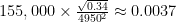
A brown dwarf’s luminosity will be negligible. To estimate its luminosity, let T be its current effective temperature in kelvins. Then:

Here, L is the brown dwarf’s luminosity in solar units.

Second Case: Main Sequence Stars

Objects with 0.08 solar masses or more will be stars. For each star, first check to see if the star system’s age is less than or equal to the star’s Main Sequence Lifespan, as determined from the Master Stellar Characteristics Table. If so, then the star is still on the main sequence and this case applies.

A main sequence star will have an effective temperature reasonably close to the Base Effective Temperature from the table for a star of that mass. The exact effective temperature will depend on the star’s exact composition, and other factors that are beyond the scope of these guidelines. Feel free to select a current effective temperature within up to 5% of the value on the table for a star of that mass.

Low-mass stars grow hotter extremely slowly, and can be considered to have the same temperature as when they formed no matter how old they are. Select an effective temperature for them without any concern for their age.

Intermediate-mass and high-mass stars change in temperature more noticeably during their main-sequence lifespan. In general, intermediate-mass or high-mass stars will tend to begin life with an effective temperature as much as 3% or 4% below the value on the table, but will reach a peak of about 2% to 3% above that value by about two-thirds of the way through their main sequence lifespan. After that, they will tend to grow cooler again, falling back to the value on the table or even slightly lower by the end of their stable lifespan. Select an effective temperature for such stars accordingly.

Round effective temperature off to three significant figures.

Main sequence stars also grow brighter over time, as temperatures in their core rise and they are forced to radiate more heat. To estimate the current luminosity for a given main-sequence star, use:

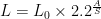
Here, L is the current luminosity for the star in solar units, L₀ is the Initial Luminosity for the star from the Master Stellar Characteristics Table, A is the star system’s age in billions of years, and S is the star’s Main Sequence Lifespan from the table. Feel free to select a final value for the star’s luminosity that is within 5% of the computed value. Round luminosity off to three significant figures.

Note that very low-mass stars have main-sequence lifespans that are far longer than the current age of the universe. Such stars have simply not had enough time to grow significantly brighter since they first formed! You may choose to simply take the Initial Luminosity for such stars without modifying it with the above computation.

Once the effective temperature and luminosity of a star have been determined, its radius can be computed. If T is a star’s effective temperature in kelvins, and L is its luminosity in solar units, then:

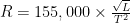
The result R is the star’s radius in AU (multiply by 150 million to get the radius in kilometers). Its diameter will be exactly twice this value. Most main-sequence stars will have radii of a small fraction of one AU.

Third Case: Subgiant and Red Giant Stars

If a given star’s age is greater than its Main Sequence Lifespan, but exceeds that value by less than 15%, then it has evolved off the main sequence and is approaching the end of its life. Such a star first evolves through a subgiant phase, during which it loses little of its brightness but grows slowly larger and cooler. At some point its core becomes degenerate, shrinking and increasing dramatically in temperature. This sets off a new form of hydrogen fusion in a shell around the core, releasing considerably more energy and causing the star’s outer layers to balloon dramatically outward. The star becomes much brighter, cooler, and larger, becoming a red giant.

Stars in this stage of their development are often somewhat unstable, and the precise path a star will follow is highly dependent on its mass, composition, and other factors. Rather than attempting to trace the star’s evolution precisely through time, we suggest simply selecting one of the three options described below. To select an option at random, roll d% on the Post-Main Sequence Table.

Post-Main Sequence Table
Roll (d%)	Stage
01-60	Subgiant
61-90	Red Giant Branch
91-00	Horizontal Branch

Subgiant stars: During this period, the star remains at about the same luminosity it had at the end of its main-sequence lifespan. Select a luminosity for the star between 2.0 and 2.4 times its Initial Luminosity from the Master Stellar Characteristics Table. The star will also cool to an effective temperature of about 5000 K. Select an effective temperature for the star somewhere between that value and the Base Effective Temperature from the table.

Red giant branch stars: At the end of the subgiant phase, a star is at the “foot” of a structure on the H-R diagram called the red giant branch. From this point, it will grow still cooler, but considerably brighter as well, swelling up to become many times its main-sequence size. The characteristics of stars at the “tip” of the red-giant branch are almost independent of the star’s mass. For stars of moderate metallicity, this implies a luminosity of about 2000 to 2500 solar units, and an effective temperature of about 3000 K.

To select an effective temperature and luminosity for a red giant branch star, select a value between 0 and 1, or roll d% to generate a random value between 0 and 1. If R is the selected value, T is the star’s current effective temperature, and L is its current luminosity, then:

Round effective temperature and luminosity to three significant figures, and feel free to select a value for each that is within 5% of the computed value.

Horizontal branch stars: Upon reaching the tip of the red giant branch, a star of moderate mass undergoes a phenomenon called helium flash. Temperatures and pressures at the star’s degenerate core have risen so high that the star can now fuse helium instead of hydrogen. A substantial portion of the star’s mass is “burned” in a few hours, releasing tremendous quantities of energy that (ironically) are almost invisible from a distance. Most of this titanic energy release is used up in lifting the star’s core out of its previously degenerate state, permitting the star to settle into a brief period of relatively stable helium burning. The star’s surface grows hotter, but it shrinks and reduces its luminosity considerably.

The temperature and luminosity of horizontal branch stars again tend to be almost independent of the star’s mass. Select a luminosity between 50 and 100 solar units, and an effective temperature of about 5000 K.

After spending a brief period on the horizontal branch, a star evolves though an asymptotic red giant phase, during which it ejects a substantial amount of its mass into space. This is the primary mechanism by which heavier elements are dispersed back into the interstellar medium, to contribute to the metallicity of later generations of stars. Asymptotic red giant stars are extremely rare, as they normally pass through that stage of their development in less than a million years. They should not be placed at random.

No matter which category the star falls into, its radius can be computed using the same formula as in the case for main sequence stars. Red giant stars are likely to be quite large, with radii of about 1 AU at their greatest extent.

Fourth Case: White Dwarf Stars

At the end of the asymptotic red giant stage, a star’s remaining core is exposed, giving rise to a stellar remnant called a white dwarf. A white dwarf is tiny, only a few thousand kilometers across, and so even if it remains extremely hot it radiates very little energy. The star’s active lifespan is now over – it no longer produces energy through nuclear fusion. Instead, the heat it retains from previous stages of its development will radiate slowly into space over billions of years.

If a given star’s age is greater than its Main Sequence Lifespan, and exceeds that value by 15% or more, then it has become a white dwarf star. As with main sequence stars, the properties of a white dwarf are strongly dependent on its mass and age.

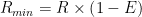
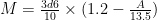
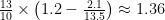
A white dwarf star is only the remnant core of a main sequence star, which will have lost a significant amount of its mass during the transition. Let M₀ be the mass of the original main sequence star, as generated in earlier steps. Then:

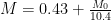
Here, M is the mass of the white dwarf remnant in solar masses. Feel free to select a value within 5% of the one computed. Replace the star’s mass, as generated in previous steps, with this result.

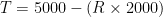
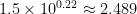
White dwarf stars are formed with very high effective temperatures, and then cool off over time as they radiate heat. To estimate the current effective temperature of a white dwarf star, let A be the age of the white dwarf (that is, the overall age of the system, minus 1.15 times the star’s Main Sequence Lifespan as taken from the Master Stellar Characteristics table). Let M be the mass of the white dwarf in solar masses, as computed above. Then:

Here, T is the white dwarf’s current effective temperature in kelvins.

The radius of a white dwarf star is almost completely determined by its mass. If M is the mass of the white dwarf, then:

Here, R is the approximate radius of the white dwarf star in kilometers. White dwarf stars are extremely small, packing a star’s mass into a sphere no larger than the Earth!

A white dwarf star’s luminosity is usually negligible, although a young (and therefore very hot) white dwarf might have a significant fraction of the Sun’s brightness. To compute a white dwarf’s luminosity, let R be its radius in kilometers and T its effective temperature in kelvins. Then:

Here, L is the star’s luminosity in solar units.

Examples

Arcadia: Alice records the values from the Master Stellar Characteristics Table for the 0.82 solar-mass primary star in the Arcadia system. It has a Base Effective Temperature of 5050 K, an Initial Luminosity of 0.28 solar units, and a Main Sequence Lifespan of 22 billion years.

The primary is 5.6 billion years old, and so is still rather early in its lifespan as a main sequence star. Alice decides to select an effective temperature for the star about 2% below the value from the table, or 4950 K. To estimate the star’s current luminosity, she uses:

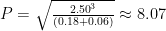
She accepts this value for the star’s luminosity, about one-third that of our Sun. To compute the star’s radius, she uses:

This gives the star’s radius in AU, which equates to a radius of about 550,000 kilometers, or about 80% that of our Sun.

Beta Nine: Bob has already determined that the Beta Nine primary star is a low-mass star with 0.18 solar masses. Since low-mass stars evolve very slowly and the whole system is only 2.1 billion years old, Bob decides to take the values for effective temperature and luminosity straight from the Master Stellar Characteristics Table, modifying each of them by less than 5% to allow for a little variety. Bob then computes the radius for the primary star using the formula under the case for main-sequence stars. For the companion, Bob computes the effective temperature and then the luminosity using the formulae under the case for brown dwarfs, and notes the fixed radius. The results are as in the table.

Beta Nine Star System
Component	Mass	Effective Temperature	Luminosity	Radius
A	0.18	3200 K	0.0045	0.001 AU
B	0.06	1420 K	0.000037	0.00047 AU

Modeling Notes

The models set out here for various stellar classes are, of course, drastically simplified for the sake of ease of use. For brown dwarfs, useful data were derived from the Burrows and Freeman papers cited below. For white dwarfs, the Catalan paper and Ciardullo’s lecture notes were most useful. Main sequence stars are the easiest to characterize, since they are the most easily observed in large numbers, so there are plenty of detailed models in existence for their properties. The Mamajek data helped to produce the Master Stellar Characteristics Table, as did the EZ-Web application for stellar modeling posted by Townsend.

Burrows, A. et al. (2001). The Theory of Brown Dwarfs and Extrasolar Giant Planets. Reviews of Modern Physics, volume 73, pp. 719-766.

Catalan, S. et al. (2008). The Initial-Final Mass Relationship of White Dwarfs Revisited: Effect on the Luminosity Function and Mass Distribution. Monthly Notes of the Royal Astronomical Society, volume 387, pp. 1692-1706.

Ciardullo, R. White Dwarf Stars. Retrieved from http://personal.psu.edu/rbc3/A414/23_WhiteDwarfs.pdf (2018).

Freeman, R. et al. (2007). Line and Mean Opacities for Ultracool Dwarfs and Extrasolar Planets. The Astrophysical Journal Supplement Series, volume 174, pp. 504-513.

Mamajek, E. A Modern Mean Dwarf Stellar Color and Effective Temperature Sequence. Retrieved from http://www.pas.rochester.edu/~emamajek/EEM_dwarf_UBVIJHK_colors_Teff.txt (2016).

Townsend, R. EZ-Web (Computer software). Retrieved from http://www.astro.wisc.edu/~townsend (2016).

Here’s the next section, a little more math-intensive, but the models are still fairly simple and straightforward. In these steps of the design sequence, the user will generate the age of the star system under development, as well as its metallicity. This last is a measure of the prevalence of heavy elements in the star system’s formation, where “heavy elements” is defined the way astronomers do, as “anything past helium on the periodic table.”

---

Step Four: Star System Age

This step determines the age of the star system being generated. All the stars in the star system will be the same age, as measured from the moment that the primary star began to fuse hydrogen in its core.

The universe is currently estimated to be 13.8 billion years old. A few stars in our Milky Way Galaxy have been determined to be about the same age, and must have formed very soon after the beginning of the universe. The Galaxy itself is not much younger than that, growing through the accretion of gas and the assimilation of smaller galaxies across billions of years.

The oldest globular clusters appear to have formed about 12.6 billion years ago, and the galactic halo must date to about the same time. Since old halo stars often have orbital paths that carry them through the galactic plane, a few of them are always likely to be found in any given neighborhood of the galactic disk. The disk itself, and the first spiral arms, appear to have formed about 8.8 billion years ago. Most stars in any given neighborhood of the disk will be younger than that.

Procedure

Select an age for the star system being generated, no greater than 13.5 billion years.

To determine an age at random, begin by rolling d% on the Stellar Age Table. Take the unmodified d% roll when generating a region of space like that of our own neighborhood (close to the plane of the Galaxy and within one of the spiral arms, but not in an active star-formation region or inside an open cluster).

Stellar Age Table
Roll (d%)	Population	Base Age	Age Range
01-05	Extreme Population I	0.0	0.5
06-31	Young Population I	0.5	2.5
32-82	Intermediate Population I	3.0	5.0
83-97	Disk Population	8.0	1.5
98-99	Intermediate Population II	9.5	2.5
00 or more	Extreme Population II	12.0	1.5

 

Population I stars are relatively young stars which make up most of the galactic disk and the spiral arms. Population II stars are old, metal-poor stars that are normally found in the galactic bulge, the galactic halo, and the globular clusters.

To determine the star system’s exact age, roll d% again, treat the result as a number between 0 and 1, multiply that number by the Age Range, and add the result to the Base Age. The result will be the age in billions of years. You may wish to round the age to two significant figures.

Selecting for an Earthlike world: Instead of determining the age completely at random, assume the star system is in the Intermediate Population I. Stars in this range of ages are most likely to be metal-rich enough to have life-bearing planets, but are also old enough for complex life to have developed there.

Examples

Arcadia: Alice wishes to determine the age of the Arcadia star system. Since she wishes the system to have at least one Earthlike world, she does not roll on the Stellar Age Table, but assumes that the star system will be Intermediate Population I. She takes a Base Age of 2.5 billion years, an Age Range of 5.0 billion years, and rolls d% for a result of 62. The age of the Arcadia system is:

Alice accepts this value for the age of the Arcadia system. The Arcadia system is apparently about a billion years older than Sol.

Beta Nine: Bob continues to work completely at random while generating the Beta Nine system. He rolls on the Stellar Age Table, getting a result of 20 on the d% roll. The Beta Nine system is in the Young Population I. He rolls another d% for a result of 82. The age of the Beta Nine system is:

Bob rounds this off to two significant figures. The Beta Nine system is 2.1 billion years old, a relatively young star system, possibly not old enough to have developed complex life.

Modeling Notes

Most surveys of the solar neighborhood suggest that there are only a few Population II stars in our vicinity. For the model in this book, we assume that this proportion is about 3% of all stars in any given region of the galactic disk. As for the younger stellar populations, astronomers tend to assume that the star-formation rate in the Galaxy has been constant for the past 8-9 billion years, which suggests a “flat” distribution of stellar ages.

Step Five: Star System Metallicity

This step determines the metallicity of the star system being generated.

Most of the matter in the universe is composed of hydrogen and helium, both of which were created in the “Big Bang” at the beginning of time. Heavier chemical elements were almost entirely created by the processes of nuclear fusion in the heart of stars. As it happens, terrestrial planets like Earth, and living beings like us, are largely made up of these heavier elements.

Early in the universe’s history, the supply of such elements was very limited, so very old stars are unlikely to have terrestrial planets capable of supporting life. However, as billions of years passed, stars “baked” the heavier elements and then scattered them back into the interstellar medium. Stars like the Sun formed in interstellar clouds of gas and dust that had been already been enriched in these heavier elements. The presence and relative abundance of these elements is what is measured by metallicity.

We will simplify by assuming that all stars in a star system have the same metallicity. This is not always observed to be the case in multiple star systems, although it is rare for members of the same multiple system to have very different metallicities.

Very old stars can have metallicity as low as zero, composed almost entirely of hydrogen and helium with only tiny traces of heavier elements. A few young stars have been located with metallicity is high as 2.5 or 3.0, with several times as great an abundance of heavy elements as the Sun. The Sun itself seems to be rather metal-rich when compared to other stars of a similar age. In general, metallicity seems to be only weakly correlated with a star’s age – even old stars can turn out to be metal-rich.

Procedure

Select a value for the star system’s metallicity. To determine metallicity at random, apply the following formula, using a roll of 3d6:

Here, M is the metallicity value, and A is the age of the star system in billions of years. Modify the result with the following two cases.

• If the star system is a member of Population II (and is therefore at least 9.5 billion years old), subtract 0.2 from the metallicity, with a minimum metallicity of 0.
• To account for the occasional unusually metal-rich star, roll 1d6. On a 1, roll 3d6 again, multiply the result by 0.1, and add it to the metallicity value, to a maximum metallicity of 3.0. This step can be applied even to very old stars.

You may wish to round metallicity to two significant figures.

Selecting for an Earthlike world: A star likely to have terrestrial planets like Earth should have a metallicity of at least 0.3. If the star’s age was selected with an Earthlike world in mind in Step Four, it is very likely to have sufficient metallicity.

Examples

Arcadia: Alice wishes to determine the metallicity of the Arcadia star system. Since she has already selected the star system’s age to try to yield at least one Earthlike world, she decides to select the metallicity value at random and see what she gets. She rolls 3d6 for a result of 8, and computes:

Rolling 1d6, she gets a value of 3, and leaves the metallicity value where it is. The Arcadia star system is rather metal-poor in comparison to our own, but it should have enough heavy elements to form terrestrial planets.

Beta Nine: Bob continues to work completely at random while generating the Beta Nine system. He rolls 3d6 for a result of 13, and computes:

Bob rounds this result off to 1.4. He then rolls 1d6 and gets a 1, indicating that the Beta Nine system formed in an unusually metal-rich region of space. He rolls 3d6 for a result of 11, and adds 1.1 to the result, for a total metallicity of 2.5. He decides that the Beta Nine system might be a good location for a mining or industrial colony.

Modeling Notes

For this book, we assume that the average metallicity of newly formed stars has been rising at a constant rate since the formation of the Galaxy. Most studies have shown that metallicity can vary widely even for stars of similar age, indicating that the distribution of heavy elements in the Galaxy is often very uneven. Data from the following paper was used to produce a rough estimate for the age-metallicity relation for stars in the solar neighborhood:

Edvardsson, B. et al. (1993). The Chemical Evolution of the Galactic Disk – Part One – Analysis and Results. Astronomy and Astrophysics, volume 275, pp. 101-152.

The next section of the star-system design sequence follows. Here, we determine whether the star system is a single or multiple star, and in the case of a multiple star we determine how many stellar components are present.

---

Step Two: Stellar Multiplicity

This step determines how many stars exist in the star system being generated.

Our own sun is a single star, traveling through the galaxy with no other stars as gravitationally bound companions. Many stars do have such companions. Double stars, gravitationally bound pairs, are very common. Multiple stars, groups of three or more stars traveling together, are much less common but do occur. Most multiple stars are trinary stars, sets of three. Sets of four or more are possible – in fact, star systems with up to seven stellar components are known – but they are quite rare.

Multiple stars are almost always found arranged in a hierarchy of pairs. That is, the stars in a system can usually be divided into pairs of closely bound partners. Each pair circles around its own center of mass, and the pairs themselves follow (usually much wider) orbital paths around the center of mass of the entire system. Any odd star is usually bound with one of the pairs. This kind of arrangement is very stable over long periods of time.

Very young multiple star systems can form trapezia, in which three or more stars follow chaotic, closely spaced paths around the system’s center of mass. This arrangement is highly unstable, and is unlikely to last very long after the stars’ original formation. Some members of a trapezium will normally be ejected, to travel as singletons. The remaining stars soon settle down into a more stable hierarchy-of-pairs arrangement.

Procedure

To begin, select whether the system being generated is a multiple star. To determine this at random, roll 3d6 and refer to the Multiplicity Threshold Table.

Multiplicity Threshold Table
Primary star’s mass (in solar masses) is . . .	Then the star is multiple on a 3d6 roll of . . .
Less than 0.08	14 or higher
At least 0.08, less than 0.70	13 or higher
At least 0.70, less than 1.00	12 or higher
At least 1.00, less than 1.30	11 or higher
At least 1.30	10 or higher

If the star system is multiple, roll d% on the Stellar Multiplicity Table. Star systems with five or more components are possible, but so rare that they should not be selected at random.

Stellar Multiplicity Table
Roll (d%)	Number of Stars
01-75	2
76-95	3
96-00	4

Selecting for an Earthlike world: Earthlike planets can appear in single or multiple star systems, although the arrangement of components in a multiple star system (determined in the next step) will affect the presence of such worlds.

Examples

Arcadia: Alice determines the multiplicity of the Arcadia star system. She knows that multiple stars might still have Earthlike worlds, but decides not to take any chances. She determines that Arcadia’s primary star will be a singleton, and does not roll on the Stellar Multiplicity Table.

Beta Nine: Bob continues to work at random while generating the Beta Nine system. He rolls 3d6 to determine whether the Beta Nine system is multiple, and gets a result of 15. Even with the primary’s star’s low mass of 0.18 solar masses, this suggests that the system will, in fact, be a multiple star system. Bob rolls d% and refers to the Stellar Multiplicity Table. His result of 46 indicates that the Beta Nine system will be a double star system.

Modeling Notes

There has been considerable recent work on the frequency of multiple star systems, leading to the (rather surprising) discovery that most stars, especially low-mass stars, are not multiple. Two of the most useful sources for this are:

Lada, C. (2006). Stellar Multiplicity and the Interstellar Mass Function: Most Stars are Single. The Astrophysical Journal Letters, volume 640, pp. 63-66.

Duchêne, G. and A. Kraus (2013). Stellar multiplicity. Annual Review of Astronomy and Astrophysics, volume 51, pp. 269-310.

Step Three: Arrange Stellar Components

This step determines how the components of a multiple star system are arranged into a hierarchy of pairs, and the initial mass of each companion star in the system. This step may be skipped if the star system is not multiple (i.e., the primary star is the only star in the system).

Astronomers normally tag the various stellar components in a multiple star system with capital letters in the Latin alphabet: A, B, C, and so on. So, for example, the famous trinary star Alpha Centauri has three components: the bright yellow-white star Alpha Centauri A, its relatively close orange companion Alpha Centauri B, and a distant red dwarf companion Alpha Centauri C (also called Proxima Centauri, since it is noticeably closer to Sol than the A-B pair).

Unfortunately, astronomers are not always consistent about which component is given which alphabetic tag. In this book, we will always tag the primary star, the most star with the highest initial mass in the system, as the A-component. The other components will be tagged in order of their distance from the primary star.

 

Procedure

The procedure for arranging stars in a system varies, depending on the multiplicity of the system.

Stars other than the primary in a multiple star system are sometimes called companion stars. These stars can have any mass, from tiny brown dwarfs up to stars almost as massive as the primary, although there is a clear tendency toward the latter.

Binary Star Systems

There is only one possible arrangement for the two stars of a binary system. There are two components, A and B, and the primary star or A-component is in a gravitationally bound pair with the B-component.

Select the mass for the companion star. To generate its mass at random, roll d% on the Companion Star Mass Table to determine a mass ratio for the companion.

Companion Star Mass Table
Roll (d%)	Mass Ratio
04 or less	0.05
05-08	0.10
09-12	0.15
13-16	0.20
17-20	0.25
21-24	0.30
25-28	0.35
31-32	0.40
35-36	0.45
37-40	0.50
41-45	0.55
46-50	0.60
51-55	0.65
56-60	0.70
61-65	0.75
66-71	0.80
72-78	0.85
79-87	0.90
88 or more	0.95

In each case, feel free to select a mass ratio that is just above the result of the table, increasing the ratio by less than 0.05. For example, if the result on the table indicates a mass ratio of 0.60, it would be appropriate to select an actual ratio greater than 0.60 but less than 0.65. The mass ratio cannot be lower than 0.05 or higher than 1.00.

In a binary star system, the companion star’s mass will be equal to the mass of the primary star, multiplied by the companion’s mass ratio. Round the companion’s mass off to the nearest hundredth of a solar mass unit. You may wish to round the companion’s mass off further, to match one of the entries in the Stellar Mass Table (see Step One). In no case will the mass of a companion star be less than 0.015 solar masses; round any such result up to that number.

Trinary Star Systems

There are two possible configurations for the three stars (components A, B, and C) of a trinary system.

One possibility is that the primary star (the A-component) has no close companion, but the B and C components move some distance away as a gravitationally bound pair of close companions (A and B-C).

The other is that the primary star and the B-component move as a bound pair of close companions, with the C-component moving alone at a greater distance (A-B and C).

Both arrangements appear to be about equally common. When designing a trinary star system, select either one. To select one at random, flip a coin.

In a trinary star system which is composed of a single A-component and a close B-C pair, the mass of the B component is computed using the Companion Star Mass Table, based on the mass of the primary star. The mass of the C-component is computed based on the mass of the B-component. When rolling on the Companion Star Mass Table, add 30 to the roll for the C component.

In a trinary star system which is composed of an A-B close pair and a C distant companion, the mass of each of the B and C components is computed using the Companion Star Mass Table, based on the mass of the primary star. When rolling on the table, add 30 to the roll for the B component.

Quaternary Star Systems

There are many possible arrangements for the four stars (components A, B, C, and D) of a quaternary system. However, by far the most common arrangement, and the most stable over long periods of time, is one in which two binary pairs (A-B and C-D) orbit one another at a wide separation.

In a quaternary star system, the mass of each of the B and C components is computed using the Companion Star Mass Table, based on the mass of the primary star. The mass of the D-component is computed based on the mass of the C-component. When rolling on the Companion Star Mass Table, add 30 to the roll for both the B component and the D component.

Examples

Arcadia: Alice skips this step for the Arcadia star system, since she already knows that the primary star is a singleton.

Beta Nine: Bob continues to work at random while generating the Beta Nine system. Since he has already established that the system is binary, he knows that there will be an A component (the primary star) and a B component (its companion). To determine the mass of the companion star, he rolls on the Companion Star Mass Table, and gets a result of 27 on the d%, for a mass ratio of 0.35. The mass of the companion star will be:

In this case, rounding the companion star’s mass off to the nearest hundredth of a solar mass unit means that it will exactly match one of the entries for brown dwarfs on the Stellar Mass Table. Bob decides to accept this result as is. The companion “star” in the Beta Nine system will be a brown dwarf.

Modeling Notes

Studies have found that the ratio of mass between the components of a binary star appears to be evenly distributed, although there seems to be a statistically significant peak for ratios of 0.95 or higher in the data.

Mass ratios seem to be somewhat dependent on the orbital period. In particular, binary pairs which orbit one another at a short distance seem more likely to be close matches in mass. For simplicity’s sake, the model set out in this book largely ignores this effect, although in trinary and higher-multiplicity star systems we do assume that the close pairs are more likely to be matched. The paper by Duchêne and Kraus (cited under Step Two) discusses these statistical phenomena in some detail.

Here’s the first section of the world-design system laid out in the Architect of Worlds project.

As a preview: the design sequence begins by walking the user through the parameters of a star system, one or more stars in a gravitationally-bound group that move together through the Galaxy. We begin by determining the mass of the primary star, which we define here as either the only star in the group, or the one that begins its life with the greatest mass. In later steps we will determine whether there are any additional stars in the system, the mass of any companion stars, the age and metallicity of the overall system, the current status of each star, and finally the orbital parameters of the system.

In later sections of the design sequence, the user will be able to place planetary systems around a given star, and design the physical parameters of individual worlds.

Readers may be a little confused as to why we’re beginning by generating the primary star’s mass. Most design sequences like this one (including at least one previous version of Architect of Worlds) start by determining how many stars are in a given system, and then move on to generate the details of each one. It turns out that a star system’s multiplicity is strongly dependent on the primary star’s mass; more massive stars are significantly more likely to appear in pairs or larger groups. That dependence is complex enough to require we take things in this order if we want plausible results.

One more thing I’d like to point out (the final book will be explicit about this): what we’re generating here is the initial mass of a given star. It’s entirely possible that the object will end up with different mass than what we have here, specifically if we find that it has aged past its red-giant phase and is now a stellar remnant. That detail will be addressed in a later step of the sequence.

---

Step One: Primary Star Mass

This step determines the initial mass of the primary star in the star system being generated. We will measure the mass of stars in solar masses.

The lowest-mass objects to be generated here are brown dwarfs, substellar objects massive enough to have planetary systems of their own, but not massive enough to sustain hydrogen fusion. Brown dwarfs are not stars, but they are sometimes referred to as such, and for the purposes of setting design they can be treated that way. Brown dwarfs have masses between about 4,000 and 25,000 times that of Earth, or between about 0.15 and 0.08 solar masses.

At 0.08 solar masses and above, objects can sustain hydrogen fusion and are considered stars. Most stars, by far, form with between 0.08 and 2.0 solar masses.

Stars can be extremely massive, up to a theoretical maximum mass of about 150 solar masses, but such gigantic stars are quite rare. Very massive stars also tend to burn through their hydrogen fuel and die very quickly, which means that they rarely get the chance to move far from the open clusters or OB associations where they were formed. Most local neighborhoods of the galaxy will have no such massive stars.

Procedure

Select a mass for the primary star of the star system being generated. To determine a mass at random, begin by rolling d% on the Primary Star Category Table.

Primary Star Category Table
Roll (d%)	Category
01-03	Brown Dwarf
04-82	Low-Mass Star
83-95	Intermediate-Mass Star
96-00	High-Mass Star

Depending on the category the primary star falls into, roll d% on the pertinent columns of the Stellar Mass Table on the next page. The result will be in solar mass units.

Feel free to select a mass for the star that is somewhere between two specific entries on the table. For example, if the result on the table indicates an intermediate-mass star of 0.92 solar masses, it would be appropriate to select an actual value greater than 0.92 but less than 0.94 solar masses. Such a selection will require you to do interpolation of several table entries in later steps.

Selecting for an Earthlike world: Instead of determining the primary star’s mass completely at random, assume it is an intermediate-mass star, and go directly to those columns on the table to determine its mass. Stars in this range are bright enough that they can have Earthlike worlds at a distance sufficient to avoid tide-locking, but are also long-lived enough that complex life is likely to have time to evolve.

Stellar Mass Table
Brown Dwarfs		Low-Mass Stars		Intermediate-Mass Stars		High-Mass Stars
Roll (d%)	Mass	Roll (d%)	Mass	Roll (d%)	Mass	Roll (d%)	Mass
01-10	0.015	01-13	0.08	01-07	0.70	01-06	1.28
11-29	0.02	14-23	0.10	08-13	0.72	07-12	1.31
30-45	0.03	24-34	0.12	14-19	0.74	13-18	1.34
46-60	0.04	35-43	0.15	20-24	0.76	19-23	1.37
61-74	0.05	44-52	0.18	25-29	0.78	24-30	1.40
75-87	0.06	53-59	0.22	30-34	0.80	31-36	1.44
88-00	0.07	60-65	0.26	35-39	0.82	37-43	1.48
		66-70	0.30	40-43	0.84	44-50	1.53
		71-74	0.34	44-47	0.86	51-58	1.58
		75-77	0.38	48-51	0.88	59-65	1.64
		78-80	0.42	52-55	0.90	66-71	1.70
		81-83	0.46	56-59	0.92	72-77	1.76
		84-86	0.50	60-62	0.94	78-84	1.82
		87-89	0.53	63-65	0.96	85-93	1.90
		90-92	0.56	66-68	0.98	94-00	2.00
		93-95	0.59	69-71	1.00
		96-97	0.62	72-74	1.02
		98-99	0.65	75-78	1.04
		00	0.68	79-82	1.07
				83-85	1.10
				85-89	1.13
				90-92	1.16
				93-95	1.19
				96-97	1.22
				98-00	1.25

Examples

Alice is aiming for a star system in which an Earthlike planet will appear, so she ignores the Primary Star Category Table and assumes the primary star will of intermediate mass. She rolls d% for a result of 36 and consults the appropriate columns on the Stellar Mass Table. The primary star’s mass is 0.82 solar masses.

Bob has no preconceived ideas about the nature of the Beta Nine system, and indeed he is designing a setting in which even small red dwarf or brown dwarf stars might be significant. He therefore rolls on the Primary Star Category Table and gets a result of 10 on the d%. The Beta Nine primary is a low-mass star. He rolls on the Stellar Mass Table, consulting the columns for low-mass stars, and gets a result of 48 on the d%. The primary star’s mass is 0.18 solar masses.

Modeling Notes

Astronomers have developed several different empirical rules for the distribution of stellar mass, each of which follows one or more power laws. In other words, the frequency of stars of a given mass seems to be proportional to that mass raised to a given power. The specific distribution we observe is called the initial mass function, and it appears to be consistent no matter where in the Galaxy we take a census of stars.

The Primary Star Category Table and Stellar Mass Table here are derived from an estimate for the initial mass function developed by the astronomer Pavel Kroupa. Citation:

Kroupa, P. (2001). On the variation of the initial mass function. Monthly Notices of the Royal Astronomical Society, volume 322, pp. 231–246.

One of my ongoing projects is a book, with the working title of Architect of Worlds. The goal of this book will be to provide science-fiction fans with the tools they need to design plausible worlds and planetary systems, using any preferred combination of random chance and deliberate selection.

From the draft Introduction for the book:

As a child in the late 1960s and early 1970s, I was fascinated by astronomy. I haunted the local library and read every book they had on the subject. I pestered my parents to plan trips to the planetarium, or to the local college when the astronomy department gave talks for the public. When I was twelve, my father purchased a high-powered telescope for me. That Celestron 8 machine saw a great deal of use over the next decade. Forty years later it is still in my possession, although (alas) I now live in a part of the country where city lights make star-gazing impractical.

I can’t be sure whether my life-long love for science fiction is a cause or an effect of that fascination with the universe around us. I grew up on stories by Asimov, Clarke, and Heinlein, and watched Star Trek re-runs at every opportunity. I was enthralled by stories of men and women going to the places I read about in my astronomy texts, discovering new worlds and meeting the strange people who lived there. I was particularly struck by authors who “showed their work” with respect to the physical environment. Authors like Poul Anderson, Hal Clement, or Larry Niven could make the settings of their stories both plausible and compelling.

At some point I discovered the world of conflict simulation games, sophisticated tabletop games that were designed to emulate various real-world political or military struggles. Most such games focused on historical conflicts, such as the American Civil War or the Second World War. A few, though, ventured into the realm of science fiction.

Almost by accident, my father brought home one such game for me, and it proved quite the revelation. This was the game Starforce, released by Simulations Publications, Incorporated in 1974.

Starforce was a simulation of human expansion into interstellar space, beginning in the twenty-fourth century. Redmond Simonsen, the game’s designer, meticulously worked out the technologies, the social and political conditions, and a complete “future history” for the game. In particular, he did careful research to build a map of space within about 20 light-years of Sol. His map included dozens of stars that could only be found in obscure astronomical catalogs, every one accurately placed.

Be it admitted, Star Trek has never worried very much about the real geography of the galaxy. Some of my favorite literary authors have done a much better job. But the fact that this game map existed – that we knew enough about our galactic neighborhood to make it possible – set my imagination alight. I spent years poring through what sources I could find, making lists of nearby stars, studying everything that was known about them, drawing maps and imagining what worlds might actually be out there.

One tool that came to my hand was another game. My father (again) came across the classic roleplaying game Traveller, and brought home a copy of the core rules for me. That game, published in 1977 by Game Designers’ Workshop, was the first to include a semi-random process for the design of star maps and worlds as settings for play. The world-building rules in the core game were very simplistic, but in the Scouts supplement (1983) a more sophisticated version appeared. This version took into account the properties of a world’s primary star, which made it possible for me to apply the system to the real stars I had been studying.

One result was the first original space-opera universe I ever designed – one which is never likely to be published, since it’s a little too obviously the result of an immature imagination. Another was a growing awareness that the Traveller rules were incomplete. To be sure, the designers produced a remarkable achievement, versions of which are still in use among Traveller players to this day. Still, they had oversimplified some details for ease of use, and the system included a few outright errors.

I set out to learn how to do better. In a sense, I’ve spent most of my adult life in that quest: a study of the universe around us, for the purpose of educating my creative imagination.

Years later, I spent about a decade writing and doing editorial work for the game publisher Steve Jackson Games. Ironically, this was at a time when they held a license to publish materials for the Traveller game and its fictional universe. That gave me the opportunity to design and publish three world-building systems of my own, which appeared in the books GURPS Traveller: First In (1999), GURPS Traveller: Interstellar Wars (2006), and GURPS Space, Fourth Edition (2006).

The last of these was the most comprehensive. It was published after the first discovery of exoplanets, worlds actually known to be circling other stars. It made an honest attempt to take into account some of the things we had already learned about the structure of planetary systems other than our own. Even so, in the years since its publication it has become dated with startling speed. In particular, the launch of the Kepler observatory in 2009 led to the discovery of hundreds of new exoplanets in just a few years. It’s become clear that the model of planetary formation I’ve used in the past was naïve at best, hopelessly wrong at worst.

Fortunately, as of this writing, the astronomical community seems to be converging on a new model, similar to the old but considerably refined. This model accounts for the great variety of exoplanets we’ve discovered, while still explaining most of the known features of our home planetary system. There is still a great deal of work to be done, and we’re likely to be surprised by what we learn in the years to come. Still, it seems possible to build a new set of world-building guidelines for the creative imagination, one which once again takes into account all that we’ve learned about the universe.

This book is intended as a resource for authors, game designers, game referees, readers, and fans of science fiction. It presents an overview of scientific concepts that might be applied to high-level design of a space-based fictional setting: the placement of stars, the arrangement of planetary systems, and the properties of individual worlds. It also presents a set of procedures for such design, allowing the reader to generate regions of space suitable for science fiction stories or games. The results should at least be plausible, given our present understanding of the universe.

More personally, this book is a collection of all the research I’ve done over the past forty years, ever since I was first inspired by those games I enjoyed as a teenager. Over the decades I’ve picked up many world-building tricks to apply in my own game writing and literary work, which I hope will be of use to others.

I’ve actually written two complete sections of Architect of Worlds, laying out how to design stars and their planetary systems. At the moment, I’m reviewing those sections and applying minor tweaks, and also ensuring that I’ve included citations to my research sources where that’s practical. I’m still working on research and development for the third major section, in which one can work out the physical details of a given world and determine what kind of environments it might support. I’m tentatively planning other sections, but those will come later.

Eventually this project is going to be compiled and sold as an e-book. One thing I plan to do with this blog is to publish an interim draft of the guidelines and systems in the book, so my readers can provide me with feedback. Entries in that series of blog entries will be posted with the architect of worlds and worldbuilding tags. Meanwhile, the book is going to be somewhat reminiscent of my work for the GURPS roleplaying game, even though it isn’t being written specifically for that game and I don’t have any reason to believe that Steve Jackson Games would be interested in publishing it. Still, I imagine GURPS fans may take a specific interest, so I’ll be posting those entries with a gurps tag as well.

Once I’ve finished posting a section of the draft here, I’ll also post a PDF of the complete section to the Sharrukin’s Archive static site. Those will eventually come down, as the book approaches readiness for publication, but that won’t be for a while.