Status Report (27 May 2018)

May 28, 2018 Sharrukin Comments 0 Comment

One of the major stumbling blocks with world-building, at least for me, is that even when I’m momentarily satisfied with the outcome of a task, it doesn’t take much to rob me of that satisfaction. In this case, while staring at my world map draft in progress, I began to compare it to both the real world and to other world-builders’ efforts, and found it lacking. Too crude.

So I’ve gone back to first principles and started over, this time rebuilding a map of tectonic plates without pre-designing any of the continental land masses. This time I strove to come up with something to resemble the general pattern of tectonic plates on the real Earth, at least as far as the number of major and minor plates was concerned. I also paid attention to the way plate boundaries are arranged – whether they tend to be convex or concave, and how they form seams and three-way intersections.

One thing I found useful was to simply mark off the polar regions and ignore those. One of the things that was giving me fits was the transformation from a flat projection to the globe and back, and that switch always introduces the most distortion close to the poles. By assuming there will be no major polar land masses, I can gloss over how any plate boundaries might be laid out in the arctic or antarctic regions.

The result (equirectangular projection only) is as follows. So far, so good. I haven’t marked continental plates yet, but there will be five major continents and a few minor land-masses and island arcs.

Next step will be mark out the relative movement of plates at each boundary, and then sketch land-forms to match.

Status Report (25 May 2018)

May 25, 2018 Sharrukin Comments 0 Comment

Just a quick report today: progress on my world maps for the Curse of Steel project. After tinkering a bit and learning how to build and use layer masks in Photoshop, I managed to paint mountain belts in their own layer on my map, with the following results:

Here, the deep-red belts are “young” mountains, the result of recent orogeny at the site of plate collisions or subduction. Think the Andes, Rockies, or Himalayas. The narrow, golden-brown belts are “old” mountains, the eroded remains of ranges that formed many millions of years ago in previous orogenic periods. Think the Appalachians or Atlas range.

One thing strikes me: the big continents to the east are going to have really big rain-shadow deserts, since those young, high mountains are going to block any kind of monsoon climate from moving too far inland. I’ll have to figure out the air circulation patterns next to know for sure. It makes sense, though, since large continents tend to have big arid zones anyway.

Next, it will be time to work out those climate patterns. I’ve been reading up on techniques for that all week, and the long weekend coming up should be a good time to work out the details.

Status Report (22 May 2018)

May 22, 2018 Sharrukin Comments 0 Comment

Had the day off sick today, so in between bouts of ick I got a bit more work done on the world map for The Curse of Steel. Mostly this involved refining the landforms, using a much finer pencil stroke to create crinkly coastlines and islands. I’m fairly happy with the results. Here’s the equirectangular base map:

Much better continental shapes, not so cartoonish now, and clear island arcs. Another view, in the Mollweide projection for variety:

Next step will be to lay out mountain ranges, in accordance with the underlying map of tectonic plates. Once that’s done, I’ll need to work out air and ocean circulation patterns, and then lay out climate zones. Then it will be time to drill down to the regional scale and build the maps I’ll need to support the story.

(Very) Rough Draft World Maps

May 21, 2018 Sharrukin Comments 0 Comment

Okay, given my level of frustration over the weekend, I’m rather happy with today’s developments. I’ve managed to produce a very rough draft of my world map, using Photoshop, the GPlates software, and GProjector. By no means is this as detailed as a good map of Earth yet, but I’m reasonably satisfied with the realism of the planetary geology involved.

Here’s a flat map in equirectangular projection:

This planet is in the middle stages of the breakup of a supercontinent. An Atlantic-like ocean has opened up, breaking off the equatorial continent and sending it south and west, creating a nice long chain of island arcs along the edges of two subduction zones as well.

The big continent that covers the north polar region is actually made up of three major continental plates. The piece covering the polar region itself is one plate, then a second is in the process of breaking away and heading southward, with a rift valley and a newly opening ocean basin dividing them. The third piece, down in the southern hemisphere, is actually a separate plate that started out attached to “Equatoria” but found itself divided from it by the new mid-ocean ridge. It’s currently being driven east and north, and is probably forming a blocked-off sea basin or an impressive range of mountains (or both) along the point of contact with the larger land mass.

The blot of land in the middle of the pseudo-Atlantic is my equivalent of Atlantis (or Númenor), the home of the most advanced human culture on the planet, one which is just starting a period of sea-borne exploration. The land-form is basically a super-Iceland, an exposed piece of the mid-ocean ridge that has a magma plume under it. Lots of volcanism and hot springs, and the inhabitants are feeling crowded enough that they’re ready to sail away and find primitive lands to colonize.

For variety, here’s a two-hemisphere orthographic map, produced using GProjector:

I did mention that this is a very rough draft map, right? I think I may produce a somewhat more detailed version of this map with Photoshop first, so I can add mountains and other major land-forms, then work out ocean currents and climate zones. Then it will be time to drill down to the specific region(s) that will appear in the story, and use Photoshop or Campaign Cartographer to put together finely detailed maps for those.

How did I get through this in just a few hours, after struggling all weekend? As often happens in world-building, the secret is finding the right workflow.

For a couple of days, I was using the GPlates software to try to draw features on the sphere. Problem is, although GPlates is perfectly good for that, that’s not what the software is actually designed for: it’s a very sophisticated plate-tectonics simulator. So by using it just to sketch features, I’m ignoring 99% of the thing’s functionality – and some of that functionality very much gets in the way. I was spending most of my time juggling multiple raster files, and fighting the very elaborate system GPlates uses to save projects, and getting frustrated with the results.

So today I switched my workflow around. Rather than do any drawing in GPlates, I did all of it in a Photoshop document with three layers (one each for ocean, tectonic boundaries, and land-masses). I would draw a few features, then save the result as a PNG image and import that into GPlates, purely to see how it looked on the sphere. More often than not, I would spot absurdities on the sphere that weren’t obvious on the flat map – so I would go back to Photoshop, fiddle with a few lines, and then re-import the result back into GPlates. I never tried to save anything in GPlates, so I never had to deal with its weird file-management system. Fifteen or twenty iterations later, I finally had the planet divided into a reasonable set of major tectonic plates, I knew where the major mid-ocean ridges and subduction zones were, and I was ready to finish the sketch map here.

I’ll take my progress where I find it.

Status Report (20 May 2018)

May 21, 2018 Sharrukin Comments 0 Comment

For the record, trying to develop a fictional planet’s geography from the plate tectonics up is a royal pain in the nether regions. I begin to see why most people just call up a noise-driven fractal map generator and call it a day.

I will persist. At the very least, I’m learning a great deal about how plate tectonics actually work. I think I may cave in and go see if anyone has developed a more detailed work-flow to make sense out of this.

Status Report (16 May 2018)

May 17, 2018 Sharrukin Comments 0 Comment

A short note, since it’s been a few days since I last posted anything here. I’ve been up to my eyebrows at the day job, teaching a course on risk management and cybersecurity. After a full day on the platform I’m rarely in good condition to get a lot of creative work done in the evening. Still, my brain has been percolating along on the Curse of Steel project.

I’m currently beginning work on some maps, to give the story some structure. The overall plot of the novel is very much in the “heroic quest” vein, with Kráva and a few companions going on a long journey across unexplored and dangerous countryside to reach an objective. So I need to at least sketch out the geography.

This, as usually happens with me, turns out to be more complicated than it might appear at first glance. Knowing too much about world-building often means you can’t be satisfied with the simple or naïve approach to any problem.

In this case, my brain got stuck on the question of how to draw regional and world maps on a sphere. I keep thinking back to the classic Baynes-Tolkien poster map of Middle-earth, which has been the inspiration for a hundred thousand fantasy-world maps since then. It’s a beautiful map, but the big unspoken problem with it is that it’s flat. The map legend indicates both constant directions and a constant distance scale, and that just cannot be done with any flat projection of a spherical surface. That’s a subtle flaw in the world-building for Middle-earth, especially if (as I suspect) Tolkien did his meticulous measurements of distance and travel times on a similarly flat map.

So, since this piece at least of my world-building is decidedly in the same mold, I want to draw a similar map – but I want to envision my world as a sphere and do my regional map-making on that basis. Which means I need to expand my cartographic tool set.

I usually do map-building with Photoshop, but it’s a challenge to draw on a sphere with that tool, and there’s no way to easily do the standard map projections. However, I’ve recently come across one of the superb world-building YouTube videos produced by Artifexian, in which he discusses a work-flow he’s developed to do just this kind of thing. Here’s a link to the specific video I’m talking about.

So I’ve gotten started on this piece of the project by downloading a couple of freeware tools (GPlates and G.Projector), and will be sketching out global and regional maps over the next few days. I’ll post some of the interim results here.

First Light for a Constructed Language

May 9, 2018 Sharrukin Comments 0 Comment

One of the occasional pitfalls I see in genre writing is the awkward use of constructed vocabulary, usually in the production of names, sometimes in the development of bits of exotic dialogue. This is usually to suggest the living language of a fantastic culture. Unfortunately, many authors are careless about this and seem to come up with their constructed vocabulary at random, so we end up with “Qadgop the Mercotan” or something equally silly. (Five kudos to anyone who recognizes the source of that name, which did in fact appear in a piece of genre fiction. At least in that case the author was trying to be silly.)

The world-building challenge is to produce an actual constructed language from which names and bits of vocabulary can emerge organically. There’s something aesthetically pleasing about this when it’s well done. The human brain seems to recognize the internal logic of a well-constructed language, even if we’re not fluent in it. J. R. R. Tolkien, of course, was the past master at this, but a lot of other authors (and hobbyists) have had a crack at it over the years.

For The Curse of Steel, I’ve decided to build at least one constructed language, mostly for naming purposes. Since I tend to insist on doing things the hard way, I’m actually building an “ur-language” and producing my primary language by applying a consistent set of sound-changes. In the back of my mind, I have half a thought that I may need a second constructed language, one that feels related to the first, rather as (e.g.) Greek and Latin are both members of the Indo-European language family. If and when I go that far, I can generate words in the second language by applying a different set of sound-changes to the ur-language roots I’ve developed.

The past few days have been fairly productive in this area. I seem to have finally developed a work-flow that actually functions, without getting me snarled up in unnecessary details of semantics, grammar, or phonology. In particular, I decided to write some text in English and “translate” that, developing new vocabulary and bits of grammar as needed. At the moment, I have about sixty words of vocabulary, several rules of inflection and word morphology, and about a page of notes on semantic structure. Enough to produce an actual paragraph of text:

Esi degra tremárakai múr kresdan. Esi kráva degraka bendír. Augrinír tan esa nekám velka devam. Enkorír skátoi taino. Antekrír skátoi tainmuro, dún begrír tan múr bákha. Vóki degra velka kresdani, dún tarthámi da skátoi. Verti kráva ked saka kó márai. Asgáni skátokai kestan, dún verti dó an atrethen degra. Rethi kráva arekhton saka padír, dún verti sa múr skáto. Dághi kráva aspera rethen skátoka klávo; esi dó kresdághen, dún esi dó degraka danpreta.

A rough back-translation into English would read something like this:

Lion was a great warrior of the Mighty People. Raven was Lion’s daughter. One night they visited the Wolf-clan. Orcs attacked the hill-fort. The orcs broke into the stockade and threatened to do great harm. Lion summoned the Wolf warriors, and opposed the orcs. Raven slew many with her bow. A chieftain of the orcs came forth, and slew Lion in single combat. Raven fought to avenge her father, and slew the great orc. After the battle, Raven took the orc’s sword, as a spoil of war and as Lion’s weregild.

You’ll recognize that as a one-paragraph summary, in pseudo-epic style, of the first chapter of The Curse of Steel, posted a few days ago here.

A few notes:

The convention in this language is to tell stories in the present tense, which is how the untranslated passage is written. In English, of course, narrative is normally framed in past tense.

The language has a very strict verb-subject-object (VSO) sentence structure. VSO languages are uncommon, although not unheard of; notably, many of the Celtic languages use that structure. It seemed appropriate, since I have a sense that Kráva’s people resemble the ancient Celts in many respects. Using a very strict word order helps with the design, since strongly positional languages don’t need quite as elaborate a system of noun or verb inflections.

I’m using a system of word roots very similar to the reconstructed Proto-Indo-European vocabulary, although in most cases I’m deliberately selecting different roots. The result should be a language that sounds as if it would be at home in the Indo-European family, without actually bearing more than a superficial resemblance to any one IE language.

A few pieces of vocabulary I’m rather pleased with:

skáto “orc” is from a word root that means “to hate,” with a noun suffix that implies a “thing” rather than a living creature or human being. Essentially, a skáto is a “thing that hates,” and notably not a person that hates. Yes, Kráva’s people really don’t like orcs.

There’s a whole vocabulary around the word kresa “war,” including kresdan “warrior” (or literally “war-man”) and kresdághen (“plunder, spoils,” literally “war-taking”). Some cultures have a hundred words for snow, but I suspect Kráva’s people may have dozens of words for armed conflict.

arekht- literally means “to set straight,” but it also carries the meanings of “to make right,” “to carry out justice,” and “to avenge.” Which probably is another clue about this culture. Related to that is the word danpreta “man-price,” or more appropriately “weregild.”

Now that I’ve been able to produce one paragraph, I can probably develop more as needed, hanging more bits of vocabulary and syntax onto the partial framework I have. I think the next piece of this project will be to start assembling a map for the story, and coming up with names for terrain features and settlements. Not sure whether I’ll do that immediately, or get back to working on Architect of Worlds again . . .

Architect of Worlds – Step Eight: Stellar Orbital Parameters

April 22, 2018 Sharrukin Comments 3 comments

This is the last step in the design sequence for star systems – once the user has finished this step, she should know how many stars are in the system, what their current properties are, and how their orbital paths are arranged.

At this point, I’ve finished the current rewrite of the “Designing Star Systems” section of the book. I don’t plan to make any further mechanical changes to that section, except to correct any errors that might pop up. The instructions and other text might get revised again before the project is complete. A PDF of the current version of this section is now available at the Sharrukin’s Archive site under the Architect of Worlds project heading.

Step Eight: Stellar Orbital Parameters

This step determines the orbital parameters of components of a multiple star system. This step may be skipped if the star system is not multiple (i.e., the primary star is the only star in the system).

Procedure

The procedure for determining the orbital parameters of a multiple star system will vary, depending on the multiplicity of the system.

The important quantities for any stellar orbit are the minimum distance, average distance, and maximum distance between the two components, and the eccentricity of their orbital path. Distances will be measured in astronomical units (AU). Eccentricity is a number between 0 and 1, which acts as a measure of how far an orbital path deviates from a perfect circle. Eccentricity of 0 means that the orbital paths follow a perfect circle, while eccentricities increasing toward 1 indicate elliptical orbital paths that are increasingly long and narrow.

Binary Star Systems

To begin, select an average distance between the two stars of the binary pair.

To determine the average distance at random, roll 3d6 on the Stellar Separation Table.

Stellar Separation Table
Roll (3d6)	Separation	Base Distance
3 or less	Extremely Close	0.015 AU
4-5	Very Close	0.15 AU
6-8	Close	1.5 AU
9-12	Moderate	15 AU
13-15	Wide	150 AU
16 or more	Very Wide	1,500 AU

To determine the exact average distance, roll d% and treat the result as a number between 0 and 1. Multiply the Base Distance by 10 raised to the power of the d% result. The result will be the average distance of the pair in AU.

Feel free to adjust the result by up to 2% in either direction. You may wish to round the result off to three significant figures.

Next, select an eccentricity for the binary pair’s orbital path. Most binary stars have orbits with moderate eccentricity, averaging around 0.4 to 0.5, but cases with much larger or smaller eccentricities are known.

To determine an eccentricity at random, roll 3d6 on the Stellar Orbital Eccentricity Table. If the binary pair is at Extremely Close separation, modify the roll by -8. If at Very Close separation, modify the roll by -6. If at Close separation, modify the roll by -4. If at Moderate separation, modify the roll by -2. Feel free to adjust the eccentricity by up to 0.05 in either direction, although eccentricity cannot be less than 0.

Stellar Orbital Eccentricity Table
Roll (3d6)	Eccentricity
3 or less	0
4	0.1
5-6	0.2
7-8	0.3
9-11	0.4
12-13	0.5
14-15	0.6
16	0.7
17	0.8
18	0.9

Once the average distance and eccentricity have been established, the minimum distance and maximum distance can be computed. Let R be the average distance between the two stars in AU, and let E be the eccentricity of their orbital path. Then:

$R_{min}=R\times\left(1-E\right)$

$R_{max}=R\times\left(1+E\right)$

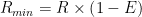
Here, R_min is the minimum distance between the two stars, and R_max is the maximum distance.

Trinary Star Systems

Whichever arrangement is selected, design the closely bound pair first as if it were a binary star system (see above). This binary pair is unlikely to have Wide separation, and will almost never have Very Wide separation. Select an average distance for the pair accordingly. If selecting an average distance at random, modify the 3d6 roll by -3. Select an orbital eccentricity normally, and compute the minimum and maximum distance for the binary pair.

Once the binary pair has been designed, determine the orbital path for the pair (considered as a unit) and the single component of the star system. The minimum distance for the pair and single components must be at least three times the maximum distance for the binary pair, otherwise the configuration will not be stable over long periods of time.

If selecting an average distance for the pair and single component at random, use the Stellar Separation Table normally. If the result indicates a separation in the same category as the binary pair (or a lower one), then set the separation to the next higher category. For example, if the binary pair is at Close separation, and the random roll produces Extremely Close, Very Close, or Close separation for the pair and single component, then set the separation for the pair and single component at Moderate and proceed.

Select an orbital eccentricity for the pair and single component normally, then compute the minimum distance and maximum distance. If the minimum distance for the pair and single component is not at least three times the maximum distance for the binary pair, increase the average distance for the pair and single component to fit the restriction.

Quaternary Star Systems

As in a trinary star system, design the closely bound pairs first. Each binary pair is unlikely to have Wide separation, and will almost never have Very Wide or Distant separation. Select an average distance for each pair accordingly. If selecting an average distance at random, modify the 3d6 roll by -3. Select an orbital eccentricity, and compute the minimum distance and maximum distance, for each binary pair normally.

Once the binary pairs have been designed, determine the orbital path for the two pairs around each other. The minimum distance for the two pairs must be at least three times the maximum distance for either binary pair, otherwise the configuration will not be stable.

If selecting an average distance for the two pairs at random, use the Stellar Separation Table normally. If either result indicates a separation in the same category as either binary pair (or a lower one), then set the separation to the next higher category. For example, if the two binary pairs are at Close and Moderate separation, and the random roll produces Moderate or lower separation for the two pairs, then set the separation for the two pairs at Wide and proceed.

Select an orbital eccentricity for the two pairs normally, then compute the minimum distance and maximum distance. If the minimum distance for the two pairs is not at least three times the maximum distance for both binary pairs, increase the average distance for the two pairs to fit the restriction.

Stellar Orbital Periods

Each binary pair in a multiple star system will circle in its own orbital period. The pair and singleton of a trinary system will also orbit around each other with a specific period (probably much longer). Likewise, the two pairs of a quaternary system will orbit around each other with a specific period.

Let R be the average distance between two components of the system in AU, and let M be the total mass in solar masses of all stars in both components. Then:

$P=\sqrt{\frac{R^3}{M}}$

Here, P is the orbital period for the components, measured in years. Multiply by 365.26 to get the orbital period in days.

Special Case: Close Binary Pairs

Most binary pairs are detached binaries. In such cases, the two stars orbit at a great enough distance that they do not physically interact with each other, and evolve independently. However, if two stars orbit very closely, it’s possible for one of them to fill its Roche lobe, the region in which its own gravitation dominates. A star which is larger than its own Roche lobe will tend to lose mass to its partner, giving rise to a semi-detached binary. More extreme cases give rise to contact binaries, in which both stars have filled their Roche lobes and are freely exchanging mass in a common gaseous envelope.

This situation is only possible for two main-sequence stars that have Extremely Close separation, or in cases where a subgiant or red giant star has a companion at Very Close or Close separation. If a binary pair being considered does not fit these criteria, there is no need to apply the following test.

For each star in the pair, approximate the radius of its Roche lobe as follows. Let D be the minimum distance between the two stars in AU, let M be the mass of the star being checked in solar masses, and let M´ be the mass of the other star in the pair. Then:

$R=D\times(0.38+0.2\log_{10}{\frac{M}{M^\prime}})$

Here, R is the radius of the star’s Roche lobe at the point of closest approach to its binary companion, measured in AU. Compare this to the radius of the star itself, as computed earlier. If the star is larger than its Roche lobe, then the pair is at least a semi-detached binary. If both stars in the pair are larger than their Roche lobes, then the pair is a contact binary.

The evolution of such close binary pairs is much more complicated than that of a singleton star or a detached binary. Mass will transfer from one star to the other, altering their orbital path and period, profoundly affecting the evolution of both. Predicting how such a pair will evolve goes well beyond the (relatively simple) models applied throughout this book. We suggest treating such binary pairs as simple astronomical curiosities, special cases on the galactic map that are extremely unlikely to give rise to native life or invite outside settlement. Fortunately, these cases are quite rare except among the very young, hot, massive stars found in OB associations.

One specific case that is of interest involves a semi-detached binary in which one star is a white dwarf. Hydrogen plasma will be stripped away from the other star’s outer layers, falling onto the surface of the white dwarf. Once enough hydrogen accumulates, fusion ignition takes place, triggering a massive explosion and ejecting much of the accumulated material into space. For a brief period, the white dwarf may shine with hundreds or even thousands of times the luminosity of the Sun. This is the famous phenomenon known as a nova.

Most novae are believed to be recurrent, flaring up again and again so long as the white dwarf continues to gather matter from its companion. However, for most novae the period of recurrence is very long – hundreds or thousands of years – so nova events from any given white dwarf in a close binary pair will be very rare. Astronomers estimate that a few dozen novae occur each year in our Galaxy as a whole.

Examples

Arcadia: Alice has already decided that the Arcadia star system has only the primary star, so she skips this step entirely.

Beta Nine: Bob knows that the Beta Nine system is a double star. Proceeding entirely at random, he rolls 3d6 on the Stellar Separation Table and gets a result of 7. The two components of the system are at Close separation. He takes a Base Distance of 1.5 AU and rolls d% for a result of 22. The average distance between the two stars in the system is:

$1.5\times{10}^{0.22}\approx2.489$

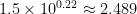
Bob rounds this off a bit and accepts an average distance of exactly 2.50 AU. He rolls 3d6 on the Stellar Orbital Eccentricity Table, subtracts 4 from the result since the stars are at Close separation, and gets a final total of 5. The orbital path of the two stars has a moderate eccentricity of 0.2. Bob computes that the minimum distance between the two stars will be 2.0 AU, and the maximum distance will be 3.0 AU.

Bob can now compute the orbital period of the two stars:

$P=\sqrt{\frac{{2.50}^3}{(0.18+0.06)}}\approx8.07$

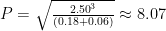
The two stars in the Beta Nine system circle one another with a period of a little more than eight years.

The two components of the Beta Nine system form a binary pair, with a minimum separation of 2.0 AU. There is no possibility of the pair forming anything but a detached binary, so Bob does not bother to estimate the size of either component’s Roche lobe.

Modeling Notes

The paper by Duchêne and Kraus cited earlier describes the best available models for the distribution of separation in binary pairs. The period of a binary star appears to show a log-normal distribution with known mode and standard deviation. Generating a log-normal distribution with dice is a challenge without requiring exponentiation at some point, hence the unusual procedure for estimating separation used here.

Architect of Worlds – Step Seven: Stellar Classification

April 19, 2018 Sharrukin Comments 0 Comment

Step Seven: Stellar Classification

This step determines the classification of each star in the system being generated, according to the Morgan-Keenan scheme most often used by astronomers. This classification scheme is not strictly necessary for the complete design of a star system, but it can provide useful flavor, and many science fiction readers and players will recognize it.

The classification for any given star is composed of two components, its spectral class and its luminosity class. Spectral class is strongly dependent on the star’s effective temperature. It uses the capital letters O, B, A, F, G, K, and M, in a sequence from the hottest (O-type) to the coolest (M-type) stars. Each letter class is also divided into ten sub-categories, numbered 0 through 9. Our own Sun, for example, is a G2-type star. Luminosity class is (for most stars) marked by a Roman numeral. Almost all stars fall into class III, class IV, or class V. Under this system, a star’s complete classification is given by spectral class, then luminosity class, with no spaces in between. Hence the Sun’s complete classification is G2V.

Brown dwarfs have also been assigned spectral classes, under an extension of the Morgan-Keenan system that uses the capital letters L, T, and Y for progressively cooler objects. These assignments are more tentative, since the study of brown dwarfs is relatively new and very cold examples are hard to observe. The spectral class Y is almost hypothetical at present, with only a few objects appearing to meet the definition.

To determine the spectral class of a star other than a white dwarf, locate the Temperature value on the Spectral Class Table closest to its effective temperature, and read across to the right to find its most likely spectral class.

Spectral Class Table
Temperature	Class	Temperature	Class	Temperature	Class	Temperature	Class
9700	A0	5900	G0	3850	M0	1300	T0
9400	A1	5840	G1	3700	M1	1200	T1
9100	A2	5780	G2	3550	M2	1100	T2
8800	A3	5720	G3	3400	M3	1000	T3
8500	A4	5660	G4	3200	M4	950	T4
8200	A5	5600	G5	3000	M5	900	T5
8000	A6	5540	G6	2800	M6	850	T6
7800	A7	5480	G7	2650	M7	800	T7
7600	A8	5420	G8	2500	M8	750	T8
7400	A9	5360	G9	2400	M9	700	T9
7200	F0	5300	K0	2300	L0	600 or less	Y0
7060	F1	5130	K1	2200	L1
6920	F2	4960	K2	2100	L2
6780	F3	4790	K3	2000	L3
6640	F4	4620	K4	1900	L4
6500	F5	4450	K5	1800	L5
6380	F6	4330	K6	1700	L6
6260	F7	4210	K7	1600	L7
6140	F8	4090	K8	1500	L8
6020	F9	3970	K9	1400	L9

Main sequence stars have a luminosity class of V. Brown dwarfs also technically fall into luminosity class V, and we will record them as such. Subgiant stars have a luminosity class of IV, and red giant stars (whether on the red giant branch or the horizontal branch) have a luminosity class of III.

White dwarf stars are an exception to this system, with their own classification scheme. We will record all white dwarf stars as having the simple classification D.

Examples

Arcadia: Alice notes that the primary star of the Arcadia system has an effective temperature of 4950 kelvins. The closest value on the Spectral Class Table is 4960 kelvins, associated with a spectral class of K2. Since the star is on the main sequence, its complete classification is K2V.

Beta Nine: Bob notes that the two stars of the Beta Nine system have effective temperatures of 3200 K and 1420 K. It turns out that the two stars are a red dwarf of class M4V and a brown dwarf of class L9V.

Modeling Notes

A star’s spectral class depends on many features of its spectrum, and when it comes to the decimal subclasses, astronomers do not agree on their definitions. The same star is often given slightly different classification depending on the source. Once again, the system described here is a simplification designed for ease of use. The primary source was Mamajek’s compiled set of definitions, cited under Step Six.

Architect of Worlds – Step Six: Stellar Evolution

April 18, 2018 Sharrukin Comments 0 Comment

This step is the core of the new design sequence for stars and stellar objects. Most world-design sequences found in tabletop games take no account of that fact that stars evolve and change over time – two stars of the same mass and composition can look very different if they are of different ages. Applying these changes to a randomly generated population of stars will provide increased plausibility, and reflect the greater variety of stars found in the real universe. This step is a trifle complex – it has four separate cases, and requires a bit more math.

Step Six: Stellar Evolution

At this point, we have determined the number of stars in the system, the initial mass of each, and the age and metallicity of the overall system. This step determines how the star system has evolved since its formation, and sets the current effective temperature, luminosity, and physical size of each star.

While on the main sequence, a star will evolve and change rather slowly, due to the “burning” of hydrogen fuel and the slow accumulation of helium “ashes” in the stellar interior. Stars normally grow brighter over time, changing in effective temperature and size as well. Stars which reach the end of their stable main-sequence lifespan go through a subgiant phase, then evolve more as a red giant, eventually losing much of their mass and settling down as a small stellar remnant called a white dwarf.

Procedure

This step should be performed for each star in a multiple star system.

Selecting for an Earthlike world: For there to be an inhabitable world in the star system, at least one star must be on the main sequence or a subgiant. If the mass and age of the primary star were selected to allow for an Earthlike world, that star is likely to fit this criterion as well.

To begin, for any object of 0.08 solar masses or more, refer to the Master Stellar Characteristics Table on the following two pages. Record the Base Effective Temperature (in kelvins) for each star. Record the Initial Luminosity (in solar units) and the Main Sequence Lifespan (in billions of years) as well.

If any star has a mass somewhere between two of the specific entries on the Master Stellar Characteristics Table, use linear interpolation to get plausible values for the star’s base effective temperature, initial luminosity, and main sequence lifespan.

Master Stellar Characteristics Table
Mass	Base Effective Temperature	Initial Luminosity	Main Sequence Lifespan
0.08	2500	0.00047	6400
0.10	2710	0.00087	4200
0.12	2930	0.0016	2800
0.15	3090	0.0029	1900
0.18	3210	0.0044	1300
0.22	3370	0.0070	870
0.26	3480	0.010	630
0.30	3550	0.013	420
0.34	3600	0.017	270
0.38	3640	0.020	170
0.42	3680	0.025	150
0.46	3730	0.031	120
0.50	3780	0.038	110
0.53	3820	0.046	92
0.56	3870	0.054	78
0.59	3940	0.065	68
0.62	4020	0.079	59
0.65	4130	0.095	51
0.68	4270	0.12	43
0.70	4370	0.13	39
0.72	4490	0.15	35
0.74	4600	0.17	32
0.76	4720	0.20	29
0.78	4830	0.22	26
0.80	4940	0.25	24
0.82	5050	0.28	22
0.84	5160	0.31	20
0.86	5270	0.35	18
0.88	5360	0.39	16
0.90	5450	0.44	15
0.92	5530	0.48	14
0.94	5590	0.53	13
0.96	5670	0.59	12
0.98	5700	0.65	11
1.00	5760	0.70	10
1.02	5810	0.78	9.3
1.04	5860	0.85	8.6
1.07	5920	0.97	7.7
1.10	5990	1.10	6.9
1.13	6030	1.30	6.5
1.16	6080	1.50	6.1
1.19	6140	1.70	5.7
1.22	6190	1.90	5.2

1.25	6250	2.10	4.7
1.28	6300	2.40	4.4
1.31	6350	2.70	4.1
1.34	6410	3.00	3.9
1.37	6470	3.30	3.6
1.40	6540	3.70	3.3
1.44	6620	4.10	2.9
1.48	6720	4.70	2.7
1.53	6870	5.50	2.5
1.58	7030	6.30	2.4
1.64	7190	7.30	2.0
1.70	7390	8.60	1.9
1.76	7550	9.90	1.6
1.82	7740	11.00	1.5
1.90	7990	14.00	1.3
2.00	8300	17.00	1.1

Once you have determined the Base Effective Temperature, Initial Luminosity, and Main Sequence Lifespan for each star in the system being designed, examine the following four cases for each star:

The first case applies to any brown dwarf with mass less than 0.08 solar masses.
The second case applies to any star with mass between 0.08 and 2.00 solar masses, if the system’s age is less than the star’s Main Sequence Lifespan. Such a star is considered a main sequence star.
The third case applies to any star with mass between 0.08 and 2.00 solar masses, if the system’s age exceeds the star’s Main Sequence Lifespan by no more than 15%. Such a star will be a subgiant or red giant star.
The fourth case applies to any star with mass between 0.08 and 2.00 solar masses, if the system’s age exceeds the star’s Main Sequence Lifespan by more than 15%. Such a star will be a white dwarf.

Apply the guidelines under the appropriate case to determine the current effective temperature, luminosity, and radius for each star.

First Case: Brown Dwarfs

A “star” with less than 0.08 solar masses will be a brown dwarf. Such an object accumulates considerable heat during its process of formation. A very massive brown dwarf may also sustain nuclear reactions in its core (deuterium or lithium burning) for a brief period after its formation, giving rise to additional heat. This heat then escapes to space over billions of years, causing the brown dwarf to radiate infrared radiation, and possibly even a small amount of visible light.

A very young and massive brown dwarf may be hard to distinguish from a small red dwarf star. Older objects will fade through deep red and violet colors, eventually ceasing to radiate visible light at all. A “dark” brown dwarf will eventually resemble a massive gas-giant planet like Jupiter. Ironically, even a very massive brown dwarf will still have about the same physical size as Jupiter, making the resemblance even stronger.

To estimate the current effective temperature of a brown dwarf, let M be the object’s mass in solar masses, and let A be the object’s age in billions of years. Then:

$T=18600\times\frac{M^{0.83}}{A^{0.32}}$

Here, T is the brown dwarf’s current effective temperature in kelvins. Effective temperature for a brown dwarf can be no higher than 3000 K.

The radius of a brown dwarf will be about 70,000 kilometers, or about 0.00047 AU.

A brown dwarf’s luminosity will be negligible. To estimate its luminosity, let T be its current effective temperature in kelvins. Then:

$L=\frac{T^4}{1.1\times{10}^{17}}$

Here, L is the brown dwarf’s luminosity in solar units.

Second Case: Main Sequence Stars

Objects with 0.08 solar masses or more will be stars. For each star, first check to see if the star system’s age is less than or equal to the star’s Main Sequence Lifespan, as determined from the Master Stellar Characteristics Table. If so, then the star is still on the main sequence and this case applies.

A main sequence star will have an effective temperature reasonably close to the Base Effective Temperature from the table for a star of that mass. The exact effective temperature will depend on the star’s exact composition, and other factors that are beyond the scope of these guidelines. Feel free to select a current effective temperature within up to 5% of the value on the table for a star of that mass.

Low-mass stars grow hotter extremely slowly, and can be considered to have the same temperature as when they formed no matter how old they are. Select an effective temperature for them without any concern for their age.

Intermediate-mass and high-mass stars change in temperature more noticeably during their main-sequence lifespan. In general, intermediate-mass or high-mass stars will tend to begin life with an effective temperature as much as 3% or 4% below the value on the table, but will reach a peak of about 2% to 3% above that value by about two-thirds of the way through their main sequence lifespan. After that, they will tend to grow cooler again, falling back to the value on the table or even slightly lower by the end of their stable lifespan. Select an effective temperature for such stars accordingly.

Round effective temperature off to three significant figures.

Main sequence stars also grow brighter over time, as temperatures in their core rise and they are forced to radiate more heat. To estimate the current luminosity for a given main-sequence star, use:

$L=L_0\times{2.2}^\frac{A}{S}$

Here, L is the current luminosity for the star in solar units, L₀ is the Initial Luminosity for the star from the Master Stellar Characteristics Table, A is the star system’s age in billions of years, and S is the star’s Main Sequence Lifespan from the table. Feel free to select a final value for the star’s luminosity that is within 5% of the computed value. Round luminosity off to three significant figures.

Note that very low-mass stars have main-sequence lifespans that are far longer than the current age of the universe. Such stars have simply not had enough time to grow significantly brighter since they first formed! You may choose to simply take the Initial Luminosity for such stars without modifying it with the above computation.

Once the effective temperature and luminosity of a star have been determined, its radius can be computed. If T is a star’s effective temperature in kelvins, and L is its luminosity in solar units, then:

$R=155,000\times\frac{\sqrt L}{T^2}$

The result R is the star’s radius in AU (multiply by 150 million to get the radius in kilometers). Its diameter will be exactly twice this value. Most main-sequence stars will have radii of a small fraction of one AU.

Third Case: Subgiant and Red Giant Stars

If a given star’s age is greater than its Main Sequence Lifespan, but exceeds that value by less than 15%, then it has evolved off the main sequence and is approaching the end of its life. Such a star first evolves through a subgiant phase, during which it loses little of its brightness but grows slowly larger and cooler. At some point its core becomes degenerate, shrinking and increasing dramatically in temperature. This sets off a new form of hydrogen fusion in a shell around the core, releasing considerably more energy and causing the star’s outer layers to balloon dramatically outward. The star becomes much brighter, cooler, and larger, becoming a red giant.

Stars in this stage of their development are often somewhat unstable, and the precise path a star will follow is highly dependent on its mass, composition, and other factors. Rather than attempting to trace the star’s evolution precisely through time, we suggest simply selecting one of the three options described below. To select an option at random, roll d% on the Post-Main Sequence Table.

Post-Main Sequence Table
Roll (d%)	Stage
01-60	Subgiant
61-90	Red Giant Branch
91-00	Horizontal Branch

Subgiant stars: During this period, the star remains at about the same luminosity it had at the end of its main-sequence lifespan. Select a luminosity for the star between 2.0 and 2.4 times its Initial Luminosity from the Master Stellar Characteristics Table. The star will also cool to an effective temperature of about 5000 K. Select an effective temperature for the star somewhere between that value and the Base Effective Temperature from the table.

Red giant branch stars: At the end of the subgiant phase, a star is at the “foot” of a structure on the H-R diagram called the red giant branch. From this point, it will grow still cooler, but considerably brighter as well, swelling up to become many times its main-sequence size. The characteristics of stars at the “tip” of the red-giant branch are almost independent of the star’s mass. For stars of moderate metallicity, this implies a luminosity of about 2000 to 2500 solar units, and an effective temperature of about 3000 K.

To select an effective temperature and luminosity for a red giant branch star, select a value between 0 and 1, or roll d% to generate a random value between 0 and 1. If R is the selected value, T is the star’s current effective temperature, and L is its current luminosity, then:

$T=5000-(R\times2000)$

$L={50}^{(1+R)}$

Round effective temperature and luminosity to three significant figures, and feel free to select a value for each that is within 5% of the computed value.

Horizontal branch stars: Upon reaching the tip of the red giant branch, a star of moderate mass undergoes a phenomenon called helium flash. Temperatures and pressures at the star’s degenerate core have risen so high that the star can now fuse helium instead of hydrogen. A substantial portion of the star’s mass is “burned” in a few hours, releasing tremendous quantities of energy that (ironically) are almost invisible from a distance. Most of this titanic energy release is used up in lifting the star’s core out of its previously degenerate state, permitting the star to settle into a brief period of relatively stable helium burning. The star’s surface grows hotter, but it shrinks and reduces its luminosity considerably.

The temperature and luminosity of horizontal branch stars again tend to be almost independent of the star’s mass. Select a luminosity between 50 and 100 solar units, and an effective temperature of about 5000 K.

After spending a brief period on the horizontal branch, a star evolves though an asymptotic red giant phase, during which it ejects a substantial amount of its mass into space. This is the primary mechanism by which heavier elements are dispersed back into the interstellar medium, to contribute to the metallicity of later generations of stars. Asymptotic red giant stars are extremely rare, as they normally pass through that stage of their development in less than a million years. They should not be placed at random.

No matter which category the star falls into, its radius can be computed using the same formula as in the case for main sequence stars. Red giant stars are likely to be quite large, with radii of about 1 AU at their greatest extent.

Fourth Case: White Dwarf Stars

At the end of the asymptotic red giant stage, a star’s remaining core is exposed, giving rise to a stellar remnant called a white dwarf. A white dwarf is tiny, only a few thousand kilometers across, and so even if it remains extremely hot it radiates very little energy. The star’s active lifespan is now over – it no longer produces energy through nuclear fusion. Instead, the heat it retains from previous stages of its development will radiate slowly into space over billions of years.

If a given star’s age is greater than its Main Sequence Lifespan, and exceeds that value by 15% or more, then it has become a white dwarf star. As with main sequence stars, the properties of a white dwarf are strongly dependent on its mass and age.

A white dwarf star is only the remnant core of a main sequence star, which will have lost a significant amount of its mass during the transition. Let M₀ be the mass of the original main sequence star, as generated in earlier steps. Then:

$M=0.43+\frac{M_0}{10.4}$

Here, M is the mass of the white dwarf remnant in solar masses. Feel free to select a value within 5% of the one computed. Replace the star’s mass, as generated in previous steps, with this result.

White dwarf stars are formed with very high effective temperatures, and then cool off over time as they radiate heat. To estimate the current effective temperature of a white dwarf star, let A be the age of the white dwarf (that is, the overall age of the system, minus 1.15 times the star’s Main Sequence Lifespan as taken from the Master Stellar Characteristics table). Let M be the mass of the white dwarf in solar masses, as computed above. Then:

$T=13500\times\frac{M^{0.25}}{A^{0.35}}$

Here, T is the white dwarf’s current effective temperature in kelvins.

The radius of a white dwarf star is almost completely determined by its mass. If M is the mass of the white dwarf, then:

$R=\frac{5500}{\sqrt[3]{M}}$

Here, R is the approximate radius of the white dwarf star in kilometers. White dwarf stars are extremely small, packing a star’s mass into a sphere no larger than the Earth!

A white dwarf star’s luminosity is usually negligible, although a young (and therefore very hot) white dwarf might have a significant fraction of the Sun’s brightness. To compute a white dwarf’s luminosity, let R be its radius in kilometers and T its effective temperature in kelvins. Then:

$L=\frac{R^2T^4}{5.4\times{10}^{26}}$

Here, L is the star’s luminosity in solar units.

Examples

Arcadia: Alice records the values from the Master Stellar Characteristics Table for the 0.82 solar-mass primary star in the Arcadia system. It has a Base Effective Temperature of 5050 K, an Initial Luminosity of 0.28 solar units, and a Main Sequence Lifespan of 22 billion years.

The primary is 5.6 billion years old, and so is still rather early in its lifespan as a main sequence star. Alice decides to select an effective temperature for the star about 2% below the value from the table, or 4950 K. To estimate the star’s current luminosity, she uses:

$0.28\times{2.2}^\frac{5.6}{22}\approx0.34$

She accepts this value for the star’s luminosity, about one-third that of our Sun. To compute the star’s radius, she uses:

$155,000\times\frac{\sqrt{0.34}}{{4950}^2}\approx0.0037$

This gives the star’s radius in AU, which equates to a radius of about 550,000 kilometers, or about 80% that of our Sun.

Beta Nine: Bob has already determined that the Beta Nine primary star is a low-mass star with 0.18 solar masses. Since low-mass stars evolve very slowly and the whole system is only 2.1 billion years old, Bob decides to take the values for effective temperature and luminosity straight from the Master Stellar Characteristics Table, modifying each of them by less than 5% to allow for a little variety. Bob then computes the radius for the primary star using the formula under the case for main-sequence stars. For the companion, Bob computes the effective temperature and then the luminosity using the formulae under the case for brown dwarfs, and notes the fixed radius. The results are as in the table.

Beta Nine Star System
Component	Mass	Effective Temperature	Luminosity	Radius
A	0.18	3200 K	0.0045	0.001 AU
B	0.06	1420 K	0.000037	0.00047 AU

Modeling Notes

The models set out here for various stellar classes are, of course, drastically simplified for the sake of ease of use. For brown dwarfs, useful data were derived from the Burrows and Freeman papers cited below. For white dwarfs, the Catalan paper and Ciardullo’s lecture notes were most useful. Main sequence stars are the easiest to characterize, since they are the most easily observed in large numbers, so there are plenty of detailed models in existence for their properties. The Mamajek data helped to produce the Master Stellar Characteristics Table, as did the EZ-Web application for stellar modeling posted by Townsend.

Burrows, A. et al. (2001). The Theory of Brown Dwarfs and Extrasolar Giant Planets. Reviews of Modern Physics, volume 73, pp. 719-766.

Catalan, S. et al. (2008). The Initial-Final Mass Relationship of White Dwarfs Revisited: Effect on the Luminosity Function and Mass Distribution. Monthly Notes of the Royal Astronomical Society, volume 387, pp. 1692-1706.

Ciardullo, R. White Dwarf Stars. Retrieved from http://personal.psu.edu/rbc3/A414/23_WhiteDwarfs.pdf (2018).

Freeman, R. et al. (2007). Line and Mean Opacities for Ultracool Dwarfs and Extrasolar Planets. The Astrophysical Journal Supplement Series, volume 174, pp. 504-513.

Mamajek, E. A Modern Mean Dwarf Stellar Color and Effective Temperature Sequence. Retrieved from http://www.pas.rochester.edu/~emamajek/EEM_dwarf_UBVIJHK_colors_Teff.txt (2016).

Townsend, R. EZ-Web (Computer software). Retrieved from http://www.astro.wisc.edu/~townsend (2016).