I’ve posted “Guanahani,” a short story that I wrote in 2015, to the Free Articles and Fiction section.
“Guanahani” is a tale about a scientific mystery, but it’s also about people trying to survive amid the perils of human history. The story should be linked from the sidebar, but here’s a link as well.
Architect of Worlds – Step Twenty: Determine Prevalence of Water
Water is one of the most common substances in the universe. Its special properties will lead it to have a profound effect on the surface conditions of any world, from its initial geological development, to its eventual climate, and finally to the evolution of life. Some worlds may never have much water, others will tend to lose whatever water they begin with, and still others will retain massive amounts of water throughout their lives.
In this step, we will estimate how much water can be found on a given world. The possible cases will be sorted into five categories: Trace, Minimal, Moderate, Extensive, and Massive. These categories are defined as follows.
Trace: No liquid water or water ice remains on the vast majority of the surface. If there is a substantial atmosphere, it may carry traces of water vapor. Small pockets of water ice may remain on the surface, in permanently shadowed craters or valleys, or on the night face of a world tide-locked to its primary star. Small deposits of water may be locked in hydrated minerals deep below the surface. Examples: Mercury, Venus, Earth’s moon, or Io.
Minimal: Liquid water is vanishingly rare on the surface, but large deposits of water ice may exist in the form of polar caps, in sheltered craters or valleys, or on the night face of a tide-locked world. Substantial aquifers or ice deposits may exist close beneath the surface. Hydrated minerals can be found in the world’s interior. Examples: Mars.
Moderate: A substantial portion of the world’s surface, but not a majority, is covered by some combination of liquid-water seas and water ice, depending on local temperature. The liquid-water oceans or ice deposits are up to a few kilometers in depth. Far away from the oceans or ice deposits, water becomes vanishingly rare. Hydrated minerals are common in the world’s interior. Examples: Mars a few billion years ago.
Extensive: Most of the world’s surface is covered by some combination of liquid-water oceans and water ice, up to several kilometers in depth. Water is common in most areas of the surface, even away from the oceans or ice deposits. Hydrated minerals are plentiful far into the world’s interior. Examples: Earth, Venus a few billion years ago.
Massive: The entire surface is covered by some combination of liquid-water oceans and water ice, up to hundreds of kilometers deep. Deeper layers of this world-ocean may be composed of higher-level crystalline forms of water (Ice II and up). Hydrated minerals are plentiful far into the world’s interior. Examples: Europa, Ganymede, Callisto, Titan, some “super-Earth” exoplanets.
The amount of water available on a given world will depend upon its M-number (Step Nineteen), its blackbody temperature (Step Nineteen), its location with respect to the protoplanetary disk (Step Nine), and (in some cases) the arrangement of any gas giant planets elsewhere in the planetary system (Steps Ten and Eleven).
Procedure
Begin by noting which of the following three cases the world being developed falls under, based on its M-number.
First Case: M-number is 2 or less
In this case, the world’s prevalence of water is automatically Massive.
Second Case: M-number is between 3 and 28
In this case, determine whether the world is outside or inside the protoplanetary nebula’s snow line, as determined in Step Nine. If the world’s orbital radius (or that of its planet, in the case of a major satellite) is exactly on the snow line, assume that it is outside.
If the world in this case is outside the snow line, then its prevalence of water is automatically Massive.
If the world in this case is inside the snow line, then roll 3d6, modified as follows:
Subtract the world’s M-number.
Add +6 if there exists a dominant gas giant in the planetary system, it experienced a Grand Tack event, and it is currently outside the protoplanetary nebula’s snow line.
Add +3 if any gas giants in the planetary system are currently outside the protoplanetary nebula’s slow-accretion line.
Take the modified 3d6 roll and refer to the Initial Water Prevalence table:
Initial Water Prevalence Table
Modified Roll (3d6)
Prevalence
-5 or less
Trace
-4 to 3
Minimal
4 to 11
Moderate
12 to 19
Extensive
20 or higher
Massive
If the result on the table is Moderate or higher, and the world’s blackbody temperature is 300 K or greater, then the presence of water vapor in the world’s atmosphere has given rise to a runaway greenhouse event. Make a note of this event for later steps in the design sequence and reduce the prevalence of water to Trace.
Otherwise (the world’s blackbody temperature is less than 300 K) the prevalence of water is as indicated on the table.
Third Case: M-number is 29 or greater
In this case, determine whether any of the three following cases is true:
The world’s blackbody temperature is 125 K or greater.
The world is the major satellite of a Large gas giant, and its orbital radius is no more than 8 times the radius of the gas giant.
The world is the major satellite of a Very Large gas giant, and its orbital radius is no more than 12 times the radius of the gas giant.
If any of these three cases are true, then the world’s prevalence of water is Trace. Otherwise, its prevalence of water is Massive.
Examples
Both Arcadia IV and Arcadia V fall into the second case. The Arcadia system has a dominant gas giant, which underwent a Grand Tack and ended up outside the snow line. The outermost gas giant (at 9.50 AU) is not outside the system’s slow-accretion line (at 14.0 AU). For both planets, therefore, she will roll 3d6, minus the planet’s M-number, plus 6. Her rolls are 13 for Arcadia IV and 10 for Arcadia V, so Arcadia IV has Extensive water while Arcadia V has only Moderate water.
Architect of Worlds – Step Nineteen: Determine Blackbody Temperature
The blackbody temperature of a world is the average surface temperature it would have if it were an ideal blackbody, a perfect absorber and radiator of heat. Real planets are not ideal blackbodies, so their surface temperatures will vary from this ideal, but the blackbody temperature is a useful tool for determining a variety of other surface conditions.
In particular, the blackbody temperature is useful in determining what atmospheric gases the world can retain over billion-year timescales. Simple thermal escape (also called Jeans escape) isn’t the only mechanism by which a world can lose atmospheric gases, but it is a strong influence on the stable mass and composition of the atmosphere.
In this step, we will compute the blackbody temperature and the M-number for the world under development. The M-number is equal to a minimum molecular weight that can be retained over long timescales.
Procedure
To determine the blackbody temperature for a world, evaluate the following:
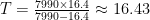
Here, L is the current luminosity of the primary star in solar units, R is the orbital radius of a planet (or the planet that a satellite orbits) in AU, and T is the blackbody temperature in kelvins. Note that the blackbody temperature will be the same for a planet and all of its satellites.
To estimate the M-number for a world, evaluate the following:
Here, T is the blackbody temperature, K is the world’s density compared to Earth, R is the world’s radius in kilometers, and M is the M-number. Round the result up to the nearest integer.
Example
Alice computes the blackbody temperature and the M-number for Arcadia IV and Arcadia V:
World
Orbital Radius
Mass
Density
Radius
Blackbody Temperature
M-Number
Arcadia IV
0.57 AU
1.08
1.04
6450 km
281 K
5
Arcadia V
0.88 AU
0.65
0.92
5670 km
226 K
6
Comparing both planets to Earth (with a blackbody temperature of 278 K and an M-number of 5), Alice finds that both of these worlds are somewhat Earthlike. Arcadia IV is just a little warmer than Earth, while Arcadia V is significantly colder.
Both worlds seem likely to have atmospheres broadly similar to that of Earth. An M-number of 5 or 6 indicates that a planet can easily retain gases such as water vapor (molecular weight 18), nitrogen (molecular weight 28), oxygen (molecular weight 32), and carbon dioxide (molecular weight 44) against simple thermal escape. It’s possible that other factors will impact the atmospheres of these worlds, but for now, Alice is satisfied that she still has two somewhat hospitable environments to use in her stories.
Still working on the next sections of Architect of Worlds.
What’s interesting is that we’re coming to a number of items that fall into a web of dependencies. Some items affect the most likely outcome of others, and it’s not a nicely linear process. Just to give you a sample, here’s some storyboarding I’ve been doing using the Miro application online:
Where this mostly comes into play is with the order that the steps need to come in the design sequence. Fortunately, I have yet to come across any dependency loops. As long as the sequence moves more or less left to right, everything should work properly . . .
Architect of Worlds – Step Eighteen: Local Calendar
In this step, we will determine elements of the local calendar on the world being developed: the length of the local day, the length of any “month” determined by a major satellite, and so on.
Length of Local Day for a Planet
To determine the length of a planet’s day – the planet’s rotation period with respect to its primary star rather than with respect to the distant stars – compute the following:
Here, P is the planet’s orbital period as determined in Step Fifteen, while R is the planet’s rotational period as determined in Step Sixteen, both in hours. T is the apparent length of the planet’s day, also in hours.
Note that this equation is undefined in cases when the orbital period and rotational period are equal (that is, the planet is in a spin-orbital resonance of 1:1 and is “tide locked”). In this case, the length of the local day is effectively infinite – the sun never moves in the sky!
At the other extreme, if the orbital period is much longer than the rotational period, then the day length and the rotational period will be very close together.
To determine the length of the local year in local days, simply divide the planet’s orbital period by the length of the local day as computed above.
Length of Apparent Orbital Period for a Satellite
To determine the length of a satellite’s orbital period, from any position on the planet’s surface, use the same equation:
Here, P is the satellite’s orbital period as determined in Step Fifteen, while R is the planet’s rotationalperiod as determined in Step Sixteen, both in hours. T is the apparent length of the satellite’s orbital period, also in hours.
Again, this equation is undefined in cases when the satellite’s orbital period and the planet’s rotational period are equal (that is, the planet is tide-locked to its satellite, or the satellite happens to orbit at a geosynchronous distance). In this case, the length of the satellite’s apparent orbital period is effectively infinite – the satellite never moves in the sky.
At the other extreme, if the satellite’s orbital period is much longer than the planet’s rotational period, then the apparent orbital period and the rotational period will be very close together. Earth’s moon is a familiar example – its apparent motion in the sky is dominated by Earth’s rotation.
It’s possible for a satellite’s orbital period to be shorter than the planet’s rotational period. For example, a moonlet that orbits very close is likely to fall into this case. The apparent orbital period will therefore be negative, indicating that the satellite appears to move backward over time. The satellite will rise in the west and set in the east.
Length of Synodic Month for a Satellite
To determine the length of a satellite’s synodic month, use the same equation once more:
Here, P is the planet’s orbital period as determined in Step Fifteen, while R is the satellite’sorbital period as determined in Step Fifteen, both in hours. T is the length of the satellite’s synodic month.
It’s very unlikely for a satellite to have the same orbital period around its planet as the planet does around its primary star, so the undefined or negative cases almost certainly will not occur. T will indicate the period between (e.g.) one “full moon” and the next, as observed from the planet’s surface.
Examples
Arcadia IV has no satellite, so the only item of interest will be the length of its local day. Alice computes:
The local day on Arcadia IV is only slightly longer than its rotation period. Alice can also determine the length of the local year in local days, by dividing the orbital period by this day length. Arcadia IV has a local year of about 184.35 local days.
Arcadia V has a satellite, so that satellite’s apparent orbital period and synodic month might be of interest. For the apparent orbital period, Alice computes:
Arcadia V’s moonlet appears to move retrograde or “backwards” in the sky, rising in the west and setting in the east, with an apparent period of about 31.7 hours.
Meanwhile, for the synodic month, Alice computes:
The satellite’s synodic month – the period between “full moon” phases – is much shorter than its apparent orbital period. From the surface of Arcadia V, the moonlet will appear to move slowly through the sky, its phase visibly changing as it moves, passing through almost a complete cycle of phases before setting once more in the east. Very strange, for human observers accustomed to the more sedate behavior of Earth’s moon!
Just a quick post today, while I continue to work on the next few steps of the Architect of Worlds design sequence. I’m noticing some renewed interest in this project, which I suppose shouldn’t surprise me given that I’m finally getting back to work on it.
It looks as if people are coming to the blog and doing a tag-search for old Architect of Worlds posts. That’s fine, but you should be aware that the earlier steps as originally posted to the blog may not be the most current version of the system. Not to mention, the blog posts aren’t always formatted so as to be easy to read or use.
For the time being, I maintain PDFs of the current “official” version of the draft on the Architect of Worlds page in the sidebar. If you’re interested in what’s been developed so far, you might want to look there rather than try to page through the old blog posts.
So long as everyone respects my copyrights, you’re welcome to download copies for your personal use. That will probably change as the book gets closer to actual publication, but that won’t be for some time yet. Of course, if you work with the system and get some interesting results, I’d be pleased to hear about that.
Architect of Worlds – Step Seventeen: Determine Obliquity
The obliquity of an object is the angle between its rotational axis and its orbital axis, or equivalently the angle between its equatorial plane and its orbital plane. It’s often colloquially called the axial tilt of a moon or planet. Obliquity can have significant effects on the surface conditions of a world, affecting daily and seasonal variations in temperature.
Procedure
Begin by noting the situation the world being developed is in: is it a major satellite of a planet, a planet with its own major satellite, or a planet without any major satellite? Notice that these three cases exactly parallel those in Step Sixteen.
First Case: Major Satellites of Planets
Major satellites of planets, as placed in Step Fourteen, will tend to have little or no obliquity with respect to the planet’s orbital plane. To determine the obliquity of such a satellite at random, roll 3d6-8 (minimum 0) and take the result as the obliquity in degrees.
Note that the major satellites of gas giants, distant from their primary star, may be an exception to this general rule. For example, in our own planetary system, the planet Uranus is tilted at almost 90 degrees to its orbital plane. Its satellites all orbit close to the equatorial plane of Uranus, so their orbits are also at a large angle, and their obliquity is very high. Cases like this are very unlikely for the smaller planets close to a primary star – tidal interactions will tend to quickly “flatten” the orbital planes of any major satellites there.
Second Case: Planets with Major Satellites
A Leftover Oligarch, Terrestrial Planet, or Failed Core which has a major satellite is likely to have its obliquity stabilized by the presence of that satellite.
To select a value of the planet’s obliquity at random, roll 3d6. Add the same modifier that was computed during Step Sixteen for the Rotation Period Table, based on the degree of tidal deceleration applied by the major satellite. Refer to the Obliquity Table.
Obliquity Table
Modified Roll
Obliquity
4 or less
Extreme (see Extreme Obliquity Table)
5
48 degrees
6
46 degrees
7
44 degrees
8
42 degrees
9
40 degrees
10
38 degrees
11
36 degrees
12
34 degrees
13
32 degrees
14
30 degrees
15
28 degrees
16
26 degrees
17
24 degrees
18
22 degrees
19
20 degrees
20
18 degrees
21
16 degrees
22
14 degrees
23
12 degrees
24
10 degrees
25 or higher
Minimal (3d6-8 degrees, minimum 0)
Feel free to adjust a result from this procedure to any value between the next lower and next higher rows on the table.
If the result is Extreme, the obliquity is likely to be anywhere from about 50 degrees up to almost 90 degrees. To select a value at random, roll 1d6 on the Extreme Obliquity Table.
Extreme Obliquity Table
Roll (1d6)
Obliquity
1-2
50 degrees
3
60 degrees
4
70 degrees
5
80 degrees
6
98-3d6 degrees, maximum 90
Again, feel free to adjust a result from this procedure to any value between the next lower and next higher rows on the table.
Third Case: Planets Without Major Satellites
A Leftover Oligarch, Terrestrial Planet, or Failed Core which has no major satellite will be most affected by its primary star.
However, without the stabilizing presence of a major satellite, the planet’s obliquity is likely to change more drastically over time. Minor perturbations from other planets in the system may lead to chaotic “excursions” of a planet’s rotation axis. For example, although at present the obliquity of Mars is about 25 degrees (comparable to that of Earth), some models predict that Mars undergoes major excursions from about 0 degrees to as high as 60 degrees over millions of years.
To select a value for obliquity at random, begin by rolling 3d6 on the Unstable Obliquity Table.
Unstable Obliquity Table
Roll (3d6)
Modifier
7 or less
Roll 1d6 – High Instability
8-13
No modifier
14 or higher
Roll 5d6 – High Instability
Make a note of any result indicating High Instability for later steps in the design sequence. The planet is likely to be undergoing drastic climate changes on a timescale of millions of years.
Now make a roll on the Obliquity Table, but if High Instability was indicated, roll 1d6 or 5d6 on this table, rather than the usual 3d6. Finally, add the same modifier that was computed during Step Sixteen for the Rotation Period Table, based on the degree of tidal deceleration applied by the primary star. Refer to the Obliquity Table, and possibly the Extreme Obliquity Table, as required.
Examples
Both Arcadia IV and Arcadia V are planets without major satellites, so they both fall under the third case in this section, as they did in Step Sixteen.
For Arcadia IV, Alice begins by rolling a 4 on the Unstable Obliquity Table, indicating that she will need to roll 1d6 rather than 3d6 on the Obliquity Table. That roll will therefore be 1d6+1, and Alice gets a final result of 3. Arcadia IV apparently has extreme obliquity in the current era. Rather than roll at random, Alice selects a value for the planet’s obliquity of about 58 degrees.
Alice makes a note of the “high instability” of the planet’s obliquity. Its steep axial tilt may be a relatively recent occurrence, taking place over the last few million years. Arcadia IV, the Earth-like candidate in her planetary system, will have very pronounced seasonal variations, and may be undergoing an era of severe climate change. Any native life has probably been significantly affected, and human colonists would need to adapt!
Meanwhile, for Arcadia V, Alice rolls a 12 on the Unstable Obliquity Table, indicating that the planet’s rotational axis is currently relatively stable. She rolls an unmodified 3d6 on the Obliquity Table, getting a result of 15. She selects a value for this planet’s obliquity of about 28.5 degrees.
Architect of Worlds – Step Sixteen: Determine Rotation Period
A quick note before I drop the next section of the draft: I caught myself making several errors in the mathematics while developing this step. I think I’ve weeded all of those out, but if anyone is experimenting with this material as it appears, let me know if you come across any odd results.
Step Sixteen: Determine Rotation Period
The next three steps in the sequence all have to do with planetary rotation. Every object in the cosmos appears to rotate around at least one axis, and in fact some objects appear to “tumble” by rotating around more than one.
Planets and their major satellites usually have simple rotation, spinning in the same direction as their orbital motion, around a single axis that is more or less perpendicular to the plane of their orbital motion. There are, of course, a variety of exceptions to this general rule.
In this step, we will determine the rotation period of a given world. In this case, we will be dealing with what’s called the sidereal period of rotation – the time it takes for a world to rotate once with respect to the distant stars.
Worlds appear to form with wildly varying rotation periods, the legacy of the chaotic processes of planetary formation. However, many worlds will have been affected by tidal deceleration applied by the gravitational influence of nearby objects. Tidal deceleration may cause a world to be captured into a special status called a spin-orbital resonance, in which the world’s orbital period and its rotational period form a small-integer ratio.
Procedure
Begin by noting the situation the world being developed is in: is it a major satellite of a planet, a planet with its own major satellite, or a planet affected primarily by its primary star?
First Case: Major Satellites of Planets
Major satellites of planets, as placed in Step Fourteen, will almost invariably be in a spin-orbit resonance state. Most models of the formation of such satellites suggest that they are captured into such a state almost immediately after their formation.
Since a major satellite’s orbit normally has very small eccentricity, the spin-orbit resonance will be 1:1. The satellite’s rotation period will be exactly equal to its orbital period.
Second Case: Planets with Major Satellites
A Leftover Oligarch, Terrestrial Planet, or Failed Core which has a major satellite may be captured into a spin resonance with the satellite’s orbit. This is actually somewhat unlikely; for example, Earth is not likely to become tide-locked to its own moon within the lifetime of the sun. However, a satellite’s tidal effects on the primary planet will tend to slow its rotation rate.
To estimate the probability that a planet has become tide-locked to its satellite, and to estimate its rotation rate if this is not the case, begin by evaluating the following:
Here, A is the age of the star system in billions of years. MS and MPare the mass of the satellite and the planet, respectively, in Earth-masses. R is the radius of the satellite, and D is the radius of the satellite’s orbit, both in kilometers.
If T is equal to or greater than 2, the planet is almost certainly tide-locked to its satellite. Its rotation period will be exactly equal to the orbital period of the satellite.
Otherwise, to generate a rotation period for the planet at random, multiply T by 12, round the result to the nearest integer, add the result to a roll of 3d6, and refer to the Rotation Period Table.
Rotation Period Table
Modified Roll (3d6)
Rotation Rate
3
4 hours
4
5 hours
5
6 hours
6
8 hours
7
10 hours
8
12 hours
9
16 hours
10
20 hours
11
24 hours
12
32 hours
13
40 hours
14
48 hours
15
64 hours
16
80 hours
17
96 hours
18
128 hours
19
160 hours
20
192 hours
21
256 hours
22
320 hours
23
384 hours
24 or higher
Resonance Established
Feel free to adjust a result from this procedure to any value between the next lower and next higher rows on the table.
The planet will be tide-locked to its satellite on a result of 24 or higher, or in any case where the randomly generated rotation rate is actually longer than the satellite’s orbital period. In these cases, again, its rotation period will be exactly equal to the orbital period of the satellite.
Third Case: Planets Without Major Satellites
A Leftover Oligarch, Terrestrial Planet, or Failed Core which has no major satellite may be captured into a spin-orbit resonance with respect to its primary star. Even if this does not occur, solar tides will tend to slow the planet’s rotation rate.
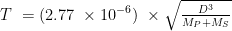
To estimate the probability that such a planet has been captured into a spin-orbit resonance, and to estimate its rotation rate if this is not the case, begin by evaluating the following:
Here, A is the age of the star system in billions of years, MS is the mass of the primary star in solar masses, MPis the mass of the planet in Earth-masses, R is the radius of the planet in kilometers, and D is the planet’s orbital radius in AU.
Again, if T is equal to or greater than 2, the planet has almost certainly been captured in a spin-orbit resonance. Otherwise, to generate a rotation period for the planet at random, multiply T by 12, round the result to the nearest integer, add the result to a roll of 3d6, and refer to the Rotation Period Table. The planet will be in a spin-orbit resonance on a result of 24 or higher, or in any case where the randomly generated rotation rate is actually longer than the planet’s orbital period.
Planets captured into a spin-orbit resonance are not necessarily tide-locked to their primary star (or, in other words, the resonance is not necessarily 1:1). Tidal locking tends to match a planet’s rotation rate to its rate of revolution during its periastron passage. If the planet’s orbit is eccentric, this match may be approximated more closely by a different resonance. To determine the most likely resonance, refer to the Planetary Spin-Orbit Resonance Table:
Planetary Spin-Orbit Resonance Table
Planetary Orbit Eccentricity
Most Probable Resonance
Rotation Period
Less than 0.12
1:1
Equal to orbital period
Between 0.12 and 0.25
3:2
Exactly 2/3 of orbital period
Between 0.25 and 0.35
2:1
Exactly 1/2 of orbital period
Between 0.35 and 0.45
5:2
Exactly 2/5 of orbital period
Greater than 0.45
3:1
Exactly 1/3 of orbital period
On this table, the “most probable resonance” is the status that the planet is most likely to be captured into over a long period of time. It’s possible for a planet to be captured into a higher resonance (that is, a resonance from a lower line on the table) but this situation is unlikely to be stable over billions of years.
Examples
Both Arcadia IV and Arcadia V are planets without major satellites, so they both fall under the third case in this section. The most significant force modifying their rotation period will be tidal deceleration caused by the primary star.
The age of the Arcadia star system is about 5.6 billion years. Arcadia IV has mass of 1.08 Earth-masses and a radius of 6450 kilometers. Alice computes T for the planet and ends up with a value of about 0.083. Arcadia IV is probably not in a spin-orbit resonance, but tidal deceleration has had a noticeable effect on the planet’s rotation. Alice rolls 3d6+1 for a result of 11 and selects a value slightly lower than the one from that line of the Rotation Period Table. She decides that Arcadia IV rotates in about 22.5 hours.
Meanwhile, Arcadia V has mass of 0.65 Earth-masses and a radius of 5670 kilometers. Alice computes T again and finds a value of about 0.007. (Notice that the amount of tidal deceleration is very strongly dependent on the distance from the primary.) Alice rolls an unmodified 3d6 for a value of 12, this time selecting a value slightly higher than the one from the table. She decides that Arcadia V rotates in about 34.0 hours.
Citations
Gladman, Brett et al. (1996). “Synchronous Locking of Tidally Evolving Satellites.” Icarus, volume 122, pp. 166–192.
Makarov, Valeri V. (2011). “Conditions of Passage and Entrapment of Terrestrial Planets in Spin-orbit Resonances.” The Astrophysical Journal, volume 752 (1), article no. 73.
Peale, S. J. (1977). “Rotation Histories of the Natural Satellites.” Published in Planetary Satellites (J. A. Burns, ed.), pp. 87–112, University of Arizona Press.
Architect of Worlds – Step Fifteen: Determine Orbital Period
So, for the first time in over two years, here is some new draft material from the Architect of Worlds project. First, some of the introductory text from the new section of the draft, then the first step in the next piece of the world design sequence.
The plan, for now, is to post these draft sections here, and post links to these blog entries from my Patreon page. None of this material will be presented as a charged update for my patrons yet. In fact, there may be no charged release in September, since this project is probably going to be the bulk of my creative work for the next few weeks. At most, I may post a new piece of short fiction as a free update sometime this month.
Designing Planetary Surface Conditions
Now that a planetary system has been laid out – the number of planets, their arrangement, their overall type, their number and arrangement of moons, all the items covered in Steps Nine through Fourteen – it’s possible to design the surface conditions for at least some of those many worlds.
In this section, we will determine the surface conditions for small “terrestroid” worlds. In the terms we’ve been using so far, this can be a Leftover Oligarch, a Terrestrial Planet, a Failed Core, or one of the major satellites of any of these. A world is a place where characters in a story might live, or at least a place where they can land, get out of their spacecraft, and explore.
Some of the surface conditions that we can determine in this section include:
Orbital period and rotational period, and the lengths of the local day, month, and year.
Presence and strength of the local magnetic field.
Presence, density, surface pressure, and composition of an atmosphere.
Distribution of solid and liquid surface, and the composition of any oceans.
Average surface temperature, with estimated daily and seasonal variations.
Presence and complexity of native life.
In this section, we will no longer discuss how to “cook the books” to prepare for the appearance of an Earthlike world. If you’ve been following those recommendations in the earlier sections, at least one world in your designed star system should have a chance to resemble Earth. However, we will continue to work through the extended example for Arcadia, focusing on the fourth and fifth planets in that star system.
Step Fifteen: Determine Orbital Period
The orbital period of any object is strictly determined by the total mass of the system and the radius of the object’s orbit. This is one of the earliest results in modern astronomy, dating back to Kepler’s third law of planetary motion (1619).
Procedure
For both major satellites and planets, the orbital period can be determined by evaluating a simple equation.
First Case: Satellites of Planets
To determine the orbital period of a planet’s satellite, evaluate the following:
Here, T is the orbital period in hours, D is the radius of the satellite’s orbit in kilometers, and MPand MS are the masses of the planet and the satellite, in Earth-masses. If the satellite is a moonlet, assume its mass is negligible compared to its planet and use a value of zero for MS.
Second Case: Planets
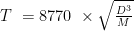
To determine the orbital period of a planet, evaluate the following:
Here, T is the orbital period in hours, D is the radius of the planet’s orbit in AU, and M is the mass of the primary star in solar masses. Planets usually have negligible mass compared to their primary stars, at least at the degree of precision offered by this equation, and so don’t need to be included in the calculation.
Examples
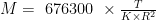
The primary star in the Arcadia system has a mass of 0.82 solar masses, and the fourth and fifth planet orbit at 0.57 AU and 0.88 AU, respectively. The two planets’ orbital periods are about 4170 hours and 7990 hours. Converting to Earth-years by dividing by 8770, the two planets have orbital periods of 0.475 years and 0.911 years.
Alice has decided to generate more details for the one satellite of Arcadia V. This is a moonlet and so can be assumed to have negligible mass, while the planet itself has a mass of 0.65 Earth-masses. The moonlet’s orbital radius is about five times that of the planet, and Alice sets a value for this radius of 28400 kilometers. The moonlet’s orbital period is about 16.4 hours.
![T=278\times\frac{\sqrt[4]{L}}{\sqrt R}](https://s0.wp.com/latex.php?latex=T%3D278%5Ctimes%5Cfrac%7B%5Csqrt%5B4%5D%7BL%7D%7D%7B%5Csqrt+R%7D+&bg=ffffff&fg=000&s=0&c=20201002)