This is the last chunk of the “design planetary systems” section of the Architect of Worlds draft. Before I post it, a small status report.
One of the things I’ve been doing over the past week is applying the current draft model to some real-world data – the HIPPARCOS catalog of the nearest stars to Sol. The next major project on my Gantt chart, after all, is to draw a map of nearby space and take a census of plausible habitable worlds in our neighborhood. This effort is helping me to test out the model, and it’s giving me data to suggest how to outline the next section (on designing specific planets).
So far, the results have actually been rather encouraging. I’ve been able to apply the model and the design sequence even to nearby stars for which we have strong candidate exoplanets. In those cases, I’ve been able to demonstrate not only that the model permits the known exoplanets, but that it also plausibly extrapolates what other planets may exist in the system, as yet undetected! That’s a good check on whether the model and design sequence are actually going to hold up against the real universe.
On the other hand, I have come across a few bits of data indicating that I need to make some revisions. In particular, the current design sequence doesn’t deal with red dwarf stars very well. I’m getting crowded arrays of Mercury- or Mars-sized rocky worlds, even in cases where what I should be seeing is icy “failed cores” out past the snow line. It’s a small logic problem, mostly in Step Eleven, which makes sense since that’s the most complex step in the sequence thus far. I think I already see how to fix it – but it will take a little bit of testing and rewriting.
I know a few of you have been experimenting with the draft sections that I’ve posted. I think what I will do, when I’ve made the necessary changes to the draft, is to revise those specific posts in place. When I’ve done that, I’ll also make a new status-report post here, with links to the altered posts. Of course, once I’m satisfied with this draft section for the time being, I’ll post a PDF to the Sharrukin’s Archive site.
Okay, with that out of the way, let’s have a look at the draft Step Fourteen.
Step Fourteen: Place Natural Satellites
In this step, we will determine the number and placement of major satellites. We define a major satellite as a natural satellite which is large enough to have formed a sphere under its own gravitation. A major satellite will be at least 200 kilometers in radius if it is mostly made of ice, or at least 300 kilometers in radius if it is mostly stone.
In general, the rocky planets close to a star are unlikely to form major satellites during the process of planetary accretion. A terrestrial planet which suffers a specific kind of massive impact event may form one major satellite, as the planetary material scattered into orbit coalesces. Gas giant planets are likely to have several major satellites. For example, planets with major satellites in our own system include Earth (1), Jupiter (4), Saturn (7), Uranus (5), and Neptune (1).
Many planets will also have moonlets, much smaller satellites that are irregular in shape. Some moonlets may be remnants of the process of planetary formation. Others are likely to be captured asteroids or comets. Even very small objects may have moonlets of their own. In our system, the planet Mars has two moonlets, and many asteroids and Kuiper Belt objects have been found to have moonlets of their own. A gas giant planet will often have dozens of moonlets in a wide variety of orbits.
Procedure
To determine the number and arrangement of natural satellites for a given planet, begin by computing the planet’s Hill radius. This is the distance from the planet within which its gravitation dominates over that of the primary star. The Hill radius defines the region of space where a satellite is likely to form or be captured, and where it can maintain a stable orbit around the planet for long periods of time.
If Rmin is the minimum distance from the planet to the primary star (in AUs), MP is the mass of the planet (in Earth-masses), and MS is the mass of the star (in solar masses), then:
![H=2170000\times R_{min}\times\sqrt[3]{\frac{M_P}{M_S}}](https://s0.wp.com/latex.php?latex=H%3D2170000%5Ctimes+R_%7Bmin%7D%5Ctimes%5Csqrt%5B3%5D%7B%5Cfrac%7BM_P%7D%7BM_S%7D%7D+&bg=ffffff&fg=000&s=0&c=20201002)
Here, H is the Hill radius in kilometers. Round off to three significant figures.
First Case: Satellites Forming via Natural Accretion
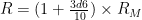
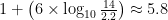
To estimate how many major satellites will form with the planet, as part of the original accretion process, evaluate the following formula:

Here, H is the Hill radius in kilometers, and R is the average distance from the planet to its primary star in AU. Round N down to the nearest integer. If the result is greater than 0, then the planet will have one or more major satellites that formed with the planet itself. No planet is likely to have more than about 8 major satellites.
If N is greater than 0, feel free to adjust N upward or downward by up to 2, so long as the result is still greater than 0 and no greater than 8. To make this adjustment at random, roll 1d6: subtract 2 from N (minimum 1) on a result of 1, subtract 1 from N (minimum 1) on a result of 2, add 1 to N (maximum 8) on a result of 5, and add 2 to N (maximum 8) on a result of 6.
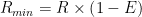
The innermost major satellite will have an orbital radius equal to about 1d+2 times the radius of the planet (feel free to adjust this by up to half the planet’s radius). Major satellites after the first can be placed using the same procedure as in Step Eleven, assuming tight orbital placement. The eccentricity of major satellite orbits will be very small (less than 0.01).
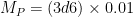
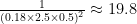
The total mass of all major satellites formed during planetary accretion will be about one ten-thousandth of the mass of the planet. The mass of each major satellite can be generated at random with a 3d6 roll:
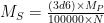
Here, MS is the mass of a major satellite in Earth-masses, MP is the mass of the planet in Earth-masses, and N is the number of major satellites. Round the satellite’s mass off to two significant figures.
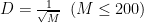
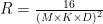
To determine the density of any of these major satellites, roll 3d6:

Here, D is the satellite’s density, and K is a constant that depends on whether the planet is inside or outside the system’s snow line. Inside the snow line, use K of 0.5. Outside the snow line, use K of 0.25. The radius and surface gravity of these major satellites can be determined as in Step Thirteen.
If a planet has one or more major satellites formed during planetary accretion, it will probably also have many moonlets. We will not generate these in detail, but they may be of interest in general.
Close to the planet will be a family of inner moonlets. These can range in number from a handful up to dozens. Their orbital radii usually range from about 1.8 times the planet’s radius, out to just inside the radius of the innermost major satellite. In some cases, inner moonlets can be interspersed between the orbits of the first few major satellites as well.
If there are inner moonlets, the planet is also likely to have a ring system. A few inner moonlets usually mean a thin system of rings, not easily visible from any distance. More inner moonlets imply a thicker and more visible set of rings. Ring systems usually hug close to the planet, reaching out to about twice the planet’s radius.
To generate the ring system at random, roll 3d6. On a result of 6-9, the planet will have a thin, wispy ring system comparable to that of Jupiter or Neptune, barely visible even at close range. On a result of 10-13, the ring system will be moderate, comparable to that of Uranus, visible from a distance through a telescope. On a result of 14 or higher, the planet will have many inner moonlets, supporting a dense ring system comparable to Saturn’s: easily visible from anywhere in the star system through a telescope, and spectacular at close range.
Beyond the major satellites will be one or more families of outer moonlets. As with the inner moonlets, these can range in number from a handful up to dozens. They are usually captured planetoids or other debris, following orbits that are eccentric, strongly inclined to the planet’s equator, or even retrograde. Their orbital radii usually begin at over 100 times the planet’s radius, and continue outward to about one-fifth to one-third of the planet’s Hill radius.
Second Case: Satellites Forming via Major Impact
Leftover Oligarchs and Terrestrial Planets, late in their formation process, are subject to repeated massive impact events. The planetary material scattered into orbit by such impacts is likely to form a large natural satellite. However, that satellite is in turn likely to spiral back into collision with the parent planet, or to migrate outward and escape the planet’s Hill radius entirely. In our own planetary system, only Earth still has a major satellite because of this process. While Mercury, Venus, and Mars all appear to have suffered similar massive impacts, none of them have retained any resulting major satellite.
To determine whether a Leftover Oligarch or Terrestrial Planet can have a large natural satellite, divide the planet’s Hill radius by its own radius. If the result is 300 or greater, then the planet can retain a large natural satellite over the long term. In this case, roll 1d: on a 5 or 6 the planet will have one large natural satellite.
If it exists, the major satellite will form quite close to the planet, but will quickly move outward due to tidal interactions. Its current orbital radius will usually be between 40 and 100 times the planet’s radius. To generate an orbital radius at random, roll 3d6+7 and multiply by 4 times the planet’s radius. The eccentricity of the major satellite’s orbit will be small (no more than about 0.05).
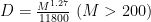
The major satellite formed by a massive impact event will have a mass about one hundredth of the mass of the planet. The mass of the major satellite can be generated at random with a 3d6 roll:

Here, MS is the mass of the major satellite, and MP is the mass of the planet, both in Earth-masses. Round the satellite’s mass off to two significant figures.
To determine the density of the major satellite, roll 3d6:

The radius and surface gravity of the major satellite can be determined as in Step Thirteen.
Third Case: Terrestrial Planet Moonlets
If a Leftover Oligarch or Terrestrial Planet has no major satellite, it may acquire one or more moonlets through a variety of means. For example, in our own planetary system, Mars has two moonlets.
A Leftover Oligarch or Terrestrial Planet may have moonlets if it can have a major satellite (that is, its Hill radius is at least 300 times the planet’s own radius) but it has no such satellite. In this case, roll 1d: on a 4-6 the planet will have at least one moonlet. Roll 1d-3 (minimum 1) for the number of moonlets.
The innermost moonlet will have an orbital radius equal to about 1d+2 times the radius of the planet (feel free to adjust this by up to half the planet’s radius). Moonlets after the first can be placed using the same procedure as in Step Eleven, assuming wide orbital placement. The eccentricity of these moonlets will be very small (less than 0.02).
Examples
Arcadia: Alice adds more columns to her table and computes the Hill radius for each planet. She then selects or randomly generates the number of major moons for each.
| Radius |
Planet Type |
Planet Mass |
Radius |
Eccentricity |
Hill Radius |
Satellites |
| 0.09 AU |
Terrestrial Planet |
0.88 |
6280 |
0.03 |
194000 |
None |
| 0.17 AU |
Terrestrial Planet |
1.20 |
6680 |
0.10 |
377000 |
None |
| 0.30 AU |
Terrestrial Planet |
0.95 |
6220 |
0.18 |
561000 |
None |
| 0.57 AU |
Terrestrial Planet |
1.08 |
6450 |
0.05 |
1290000 |
None |
| 0.88 AU |
Terrestrial Planet |
0.65 |
5670 |
0.02 |
1730000 |
1 moonlet |
| 1.58 AU |
Leftover Oligarch |
0.10 |
3380 |
0.38 |
1050000 |
2 moonlets |
| 2.61 AU |
Planetoid Belt |
N/A |
N/A |
0.00 |
N/A |
N/A |
| 4.40 AU |
Large Gas Giant |
480 |
83000 |
0.00 |
79900000 |
7 major satellites |
| 5.76 AU |
Medium Gas Giant |
120 |
70000 |
0.00 |
65900000 |
4 major satellites |
| 9.50 AU |
Small Gas Giant |
22 |
30000 |
0.08 |
56800000 |
2 major satellites |
As it happens, none of the first four inner planets can have major satellites or moonlets. In particular, the habitable-planet candidate has too small a Hill radius to permit it. Alice rolls at random for the fifth and sixth planets, and gets the results she tabulated above. She decides not to bother generating these moonlets in detail, unless her story visits one of these two planets.
With very wide Hill radii and plenty of distance between them and the primary star, the three gas giants all have extensive systems of satellites. Alice uses the formula and a random die roll to determine how many major satellites each planet has. She doesn’t bother to set up their systems of moonlets, although she does roll at random to see whether either planet has a prominent ring system. She rolls a 10, an 11, and another 10, so all three gas giants have ring systems that are visible at a distance through telescopes, but none of them have a remarkable Saturn-like set of rings.
Beta Nine: Bob computes the Hill radii for his two planets. The inner planet has a Hill radius of about 863,000 kilometers, which is only about 160 times the planet’s radius. The outer planet has a Hill radius of about 1.42 million kilometers, which is better but still comes to only about 260 times the planet’s radius. Bob concludes that neither planet has any satellites.
![D=(0.90+\frac{\left(3d6\right)}{100})\times\sqrt[5]{M}](https://s0.wp.com/latex.php?latex=D%3D%280.90%2B%5Cfrac%7B%5Cleft%283d6%5Cright%29%7D%7B100%7D%29%5Ctimes%5Csqrt%5B5%5D%7BM%7D+&bg=ffffff&fg=000&s=0&c=20201002)
![D=(0.50+\frac{\left(3d6\right)}{100})\times\sqrt[5]{M}](https://s0.wp.com/latex.php?latex=D%3D%280.50%2B%5Cfrac%7B%5Cleft%283d6%5Cright%29%7D%7B100%7D%29%5Ctimes%5Csqrt%5B5%5D%7BM%7D+&bg=ffffff&fg=000&s=0&c=20201002)
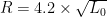
![R=6370\times\sqrt[3]{\frac{M}{D}}](https://s0.wp.com/latex.php?latex=R%3D6370%5Ctimes%5Csqrt%5B3%5D%7B%5Cfrac%7BM%7D%7BD%7D%7D+&bg=ffffff&fg=000&s=0&c=20201002)
![G=\sqrt[3]{MD^2}](https://s0.wp.com/latex.php?latex=G%3D%5Csqrt%5B3%5D%7BMD%5E2%7D+&bg=ffffff&fg=000&s=0&c=20201002)


 , as discussed under Step Ten.
![R=(2d6)\times0.01\times\sqrt[3]{M}](https://s0.wp.com/latex.php?latex=R%3D%282d6%29%5Ctimes0.01%5Ctimes%5Csqrt%5B3%5D%7BM%7D+&bg=ffffff&fg=000&s=0&c=20201002)
![R=(2d6)\times0.04\times\sqrt[3]{M}](https://s0.wp.com/latex.php?latex=R%3D%282d6%29%5Ctimes0.04%5Ctimes%5Csqrt%5B3%5D%7BM%7D+&bg=ffffff&fg=000&s=0&c=20201002)


![R=(2d6)\times0.003\times\sqrt[3]{M}](https://s0.wp.com/latex.php?latex=R%3D%282d6%29%5Ctimes0.003%5Ctimes%5Csqrt%5B3%5D%7BM%7D+&bg=ffffff&fg=000&s=0&c=20201002)
![R=15\times\sqrt[3]{M}](https://s0.wp.com/latex.php?latex=R%3D15%5Ctimes%5Csqrt%5B3%5D%7BM%7D+&bg=ffffff&fg=000&s=0&c=20201002)